Ffowcs Williams & Hawkings Analogy

Error

This treatment is provided by an external module and is not part of the core system. If you’re interested in accessing or utilizing this feature, please contact us for further details and support.

Description

This treatment predicts the fluctuating pressure in far-field using the Ffowcs Williams & Hawkings Analogy. The formulation 1A (Farassat 2007) and the formulation 1C (Najafi-Yazdi 2011) are available for both static surfaces and surfaces in a rotating frame of reference. The advanced time approach (Casalino, 2003) is used for the prediction of acoustic fields. Variants of the Ffowcs Williams - Hawkings equation introduced by Morfey in 2007 and Shur in 2005 are also available (Spalart 2009). The mean flow is assumed to be along the \(\vec{x}\) direction, if not the reference frame must be rotated to satisfy this condition.

The interested reader can make reference to the papers of Casalino (2003) and Najafi-Yazdi et al. (2011).

The FW-H acoustic analogy involves enclosing the sound sources with a control surface that is mathematically represented by a function, \(f (\mathbf{x}, t)=0\). The acoustic signature at any observer position can be obtained from the FW-H equation:

\[\begin{aligned} p ^ { \prime } ( \mathbf { x } , t ) = \frac { \partial } { \partial t } \int _ { f = 0 } \left[ \frac { Q _ { i } n _ { i } } { 4 \pi | \mathbf { x } - \mathbf { y } | } \right] _ { \tau _ { e } } \mathrm { d } S - \frac { \partial } { \partial x _ { i } } \int _ { f = 0 } \left[ \frac { L _ { i j } n _ { j } } { 4 \pi | \mathbf { x } - \mathbf { y } | } \right] _ { \tau _ { \mathrm { e } } } \mathrm { d } S + \frac { \partial ^ { 2 } } { \partial x _ { i } \partial x _ { j } } \int _ { f > 0 } \left[ \frac { T _ { i j } } { 4 \pi | \mathbf { x } - \mathbf { y } | } \right] _ { \tau _ { \mathrm { e } } } \mathrm { d } V \end{aligned}\]

where \([ ]_{\tau_e}\) denotes evaluation at the emission time \(\tau_e\). and \(V\) represents the volume outside the control surface. The source terms under the integral sign are:

\[\begin{split}\begin{aligned} Q _ { i } & = \rho \left( u _ { i } - v _ { i } \right) + \rho _ { 0 } v _ { i } \\ L _ { i j } & = \rho u _ { i } \left( u _ { j } - v _ { j } \right) + P _ { i j } \end{aligned}\end{split}\]

and \(T_{ij}\) is referred to as Lighthill’s stress tensor:

\[T _ { i j } = \rho u _ { i } u _ { j } + \left[ \left( p - p _ { 0 } \right) - c _ { 0 } ^ { 2 } \left( \rho - \rho _ { 0 } \right) \right] \delta _ { i j } - \sigma _ { i j }\]

The vectors \(\mathbf{u}\) and \(\mathbf{v}\) are the flow and the surface velocities, respectively. The compression tensor \(P_{ij}\) is defined as:

\[P _ { i j } = \left( p - p _ { 0 } \right) \delta _ { i j } - \sigma _ { i j }\]

The three source terms in the formal definition of \(p ^ { \prime } ( \mathbf { x } , t )\) are known as the thickness (\(Q _ { i }\), monopole), loading (\(L _ { ij }\), dipole) and quadrupole (\(T _ { ij }\)) source terms, respectively.

Features

• Farassat 1A in a medium at rest.

• Convective Nayafi-Yasdi 1C (with mean flow).

• Both unstructured & structured surfaces.

• Static surfaces and surfaces with a rotating frame of reference.

• Porous and solid formulations.

• Multi-code tool, tested and validated on:

  • AVBP

  • elsA

  • ProLB

  • Cosmic (University of Leicester)

  • FLUSEPA

Parameters

• base: Base, default= None

  The surface base on which the FWH surface integral will be computed. It can contain several zones and several instants. The object will be modified at the output.

• meshfile: list(str), default= None

  A two element list or tuple containing, first the name of the meshfile, followed by the reader format used to read the mesh.

• datafile: list(str), default= None

  A two element list or tuple containing, first the name of the datafile, followed by the reader format used to read the data.

  Warning

  This keyword only works if the base is written such as every instant is stored in a different file.

• modify_surface: function, default= None

  A function used to modify the FWH surface at runtime. See here for more details.

• coordinate_names: list(str), default= None

  A three element list or tuple containing the name variable of spatial coordinates. If None, the names will be inferred from the database using the antares.Constants.KNOWN_COORDINATES list.

• surface_normal_components: list(str), default= None

  A three element list or tuple containing the variable name of the three surface normal components.

• compute_normal_vectors: function, default= None

  The function used to compute the surface normal vectors and align them in the right direction. See Compute normal vectors for more details. Additionally, FWH Utils offers a few functions that can be used to compute the normal vectors in most scenarios.

• redim: list(float), default= None

  A list of 6 floats used to convert the following values: length, density, velocity, pressure, temperature, and time.

• volume_base: Base, default= None

  The volume base on which the FWH volume integral will be computed. It can contain several zones and several instants. The object will be modified at the output.

• volume_meshfile: list(str), default= None

  A two element list or tuple containing, first the name of the volume meshfile, followed by the reader format used to read the mesh.

• volume_datafile: list(str), default= None

  A two element list or tuple containing, first the name of the datafile containing the volume base, followed by the reader format used to read the data.

  Warning

  This keywords only works if the base is written such as every instant is stored in a different file

• modify_volume: function, default= None

  A function used to modify the FWH volume at runtime. See here for more details.

• pressure_variable: str, default= ‘pressure’

  A string containing the name of the pressure variable.

• pressure_equation: str, default= None

  A string containing an equation to compute the pressure from the variables present in the base.

• velocity_variables: list(str), default= None

  A list of strings containing the name of the velocity components.

• velocity_equations: list(str), default= None

  A list of strings containing the equations to compute the velocity variables from the variables present in the base.

• density_variable: str, default= None

  A string containing the name of density variable.

• density_equation: list(str), default= None

  A string containing an equation to compute the density variable from the variables present in the base.

• obs_file: str

  A column-type file defining the position for each observer in the far-field. The base must contain the variables 'x', 'y', and 'z'.

• type: str, default= porous

  The type of acoustic analogy formulation: 'porous' or 'solid'.

• analogy: str, default= 1A

  Acoustic analogy formulation: '1A' or '1C'.

• form: str, default= density

  Form of the acoustic analogy (pressure or density based):

  • 'density' stand for the original FW-H formulation: \(\rho' = \rho - \rho_0\)

  • 'pressure1' stand for the Morfey modification: \(\rho^{\star} = \rho_0 + p/c_0^2\)

  • 'pressure2' stand for Shur modification: \(\rho^{\diamond} = \rho_0 (1+p/p_0)^{1/\gamma}\)

• quadrupole_term: str, default= None

  • None: do not compute the quadrupole term.

  • 'full': compute the volume + surface integrals (a volume base must be specified).

  • 'only': compute only the volume integral (a volume base must be specified).

  • 'cancel_spurious_noise': compute the quadrupole surface correction following the model of Rahier et al. (2015)

  • 'frozen_turbulence': compute the quadrupole surface correction following the model of Ikeda et al. (2017)

• eddy_convective_velocity: str, default= None

  The type of eddy convective velocity needed to compute the 'frozen_turbulence' quadrupole correction term

  • 'temporal_mean': velocity time average.

  • 'mean_flow': mean flow in the x direction.

• pref: float, default= 101325.0

  The value of the reference pressure in Pa.

• tref: float, default= 298.0

  The value of the reference temperature in K.

• mach: float, default= 0.0

  Ambient medium Mach number for analogy 1C.

• R_gas: float, default= 287.058

  Mass-specific gas constant in J/(Kg K) = m2/(s2 K).

• gamma: float, default = 1.4

  Heat capacity ratio ( \(c_p / c_v\) ).

• mesh_kinetics: str, default = static

  Describes the type of movement of the mesh. Two possible values:

  • 'static': a static mesh.

  • 'rotating_reference_frame': a mesh with a rotating reference frame. The angular velocity and the rotation axis are assumed to be constant.

• rotation_velocity: float, default = 0

  Angular velocity in rad/s for a mesh in a rotating reference frame.

• rotation_axis: list(float), default = [0, 0, 0]

  The direction of the rotation axis of a mesh in a rotating reference frame.

• dt: float, default= None

  Simulation time step.

• sample: int, default= 1

  The number of time steps between two instants. The \(\Delta t\) between two instants should be equal to \(dt \times \text{sample}\).

• start_propagation_at: float, default = None

  The physical time with respect to the source at which the FWH propagation should start. If None the propagation starts from the first instant in the database.

• end_propagation_at: float, default = None

  The physical time with respect to the source at which the FWH propagation should end. If None the propagation will be performed until the last instant in the database.

• initial_time: float, default = 0.0

  The physical time of the first instant in the database.

• nb_revolutions: int, default= 1

  Number of extra revolutions to be propagated. This assumes that the database contains only one revolution or a partial revolution and partial_periodicity is set to True.

• partial_periodicity: bool, default= False

  If False, the input base is assumed to contain a full 360 \(^o\) revolution. If True, the input base is assume to contain a partial part of a full rotation and the missing parts are assumed to be periodic with respect to the input base.

• derivative_order: int, default= 1,

  Order of the finite difference scheme used to compute the time derivatives.

• output: str, default= fwh_result

  Output file name (hdf_antares format).

• output_contributions: bool, default= False

  It True, the output base will contain the individual thickness loading and quadrupole noise contributions.

• verbose: bool, default= True

  If True, the output will print the information of the treatment progress and performance. If False, nothing will be printed.

Preconditions

The following conditions must be met in order to ensure a correct execution of the treatment:

• The treatment depends on mpi4py (even if run without MPI).

• All the zones must have the same number of instants.

• In case of a single zone base, all the cell elements must be of the same type.

• The observer file must be in a 'column' format.

• The mean flow is assumed to be along the \(\vec{x}\) direction. If not, the reference frame must be rotated to satisfy this condition.

• The rotation axis is assumed to pass by the origin of the reference frame. If not, the reference frame must be translated to satisfy this condition.

• The rotation axis direction must not be the zero vector when mesh_kinetics = 'rotating_reference_frame'.

• The mesh topology is assumed to be constant when mesh_kinetics = 'rotating_reference_frame'.

Postconditions

The output base contains \(N+1\) zones where \(N\) is the number of observers. By convention, the first zone contains one instant with only one variable, the time vector common to all observers. The rest of the zones contain the information for each observer. They all contain also one instant with the pressure related variables and the convergence vector.

The base also stores useful information in its attributes. The base level attributes contain the information of the value of all keywords used in the treatment (including the default ones). If the value of a keyword is an antares.Base, the stored attributes will be the string “User defined”. If the value of a keyword is a function, only the name of the function will be saved in the attributes.

If the library GitPython is installed in the system, the following attributes will be saved:

• The path to the antares repository.

• The name of the current branch.

• The SHA of the latest commit.

• If the repository is in a dirty state (A git repo is dirty if there are modified tracked files and/or staged changes, but untracked content doesn’t count)

Additionally, several system related information is also saved in the attributes such as:

• The host system information as provided by the platform.uname() function.

• The path and version of the current python binary.

• The current working directory.

• The name and arguments of the main script.

• The date at which the treatment ended.

• The CPU time.

• The number of MPI procs used.

• The path of the script containing the FWH treatment.

Furthermore, the zone level attributes store the spatial coordinates for each observer in the variables “x”, “y”, and “z”.

Write a file in hdf_antares format (default: fwh_result.h5).

Modify surface and volume databases

This treatment allows the user to modify the database at run-time. This could allow the user to modify the geometry on which perform the FWH treatment (by removing nodes, zones, etc). This can also be used to modify the physical variables in a more complex way than what it is allowed with the redim or equations keywords

For performance reasons, this modification is not done over the whole database at once, but one instant at a time during the FWH main execution loop. This reduces the memory footprint of the treatment as the whole database will not be uploaded into memory. This also allows to implement some additional performance optimizations.

The modification is done by using the functions provided by the user using the modify_surface and modify_volume keywords. These keywords require as value a function that accepts 3 arguments:

1. base: An antares.Base with only one instant (the instant currently being processed).

2. it: an integer containing the current iteration index starting from 0.

3. user_defined_vars: a dictionary in which the user can store any variable to be re-used for future iterations.

A skeleton and usage of this function is shown below:

import antares

def modify_surface(base: antares.Base,
                   it: int,
                   user_defined_vars):

    # Modify base
    new_base = # ...

    # return modified base
    return new_base

treatment = antares.Treatment('fwh')
treatment['modify_surface'] = modify_surface
# .
# .
# .
treatment.execute()

Internally, the FWH treatment stores the geometric and the physical variables in different bases. If mesh_kinetics is either 'static' or 'rotating_reference_frame', the variable geometry is taken from the output of the modify_surface function at it=0. Trying to modify the geometric variables for it>0 will have no effect.

Warning

The treatment does not check that the modification applied to the base are consistent with what the treatment needs.

The user must ensure consistency between all the instants and the geometry. This is especially true when trying to remove nodes, cells or zones. They must be removed from each instant.

Compute normal vectors

In order to correctly propagate the noise using the FWH analogy, the normal vectors of the FWH surface must be computed. These vectors must point outwards. If the vector components are already present in the original database, then the user can use surface_normal_components keywords to indicate the variable names. If they are not present in the database, the user should use the compute_normal_vectors to compute the normal vectors, already pointing outwards.

This keywords accepts a function of 3 arguments:

1. geometry: an antares.Base with as many zones as the original input database, and only one instant containing the spatial coordinates as variables.

2. it: an integer representing the current iteration in the FWH loop

3. coord_names: a list of 3 strings with the names of the spatial coordinates

And the function must return a list with the names of the 3 variables representing the normal vectors components.

A skeleton of implementation and usage of this function is shown below:

import antares
from typing import List

def compute_normals(geometry: antares.Base,
                    it: int,
                    coord_names: List[str]):

    # Compute normal vectors for all zones
    for zone in geometry.keys():
        geometry[zone][0]['normal_x'] = # ...
        geometry[zone][0]['normal_y'] = # ...
        geometry[zone][0]['normal_z'] = # ...

    # return the name of the newly created variables storing the normal vector components
    return ('normal_x', 'normal_y', 'normal_z')

treatment = antares.Treatment('fwh')
treatment['compute_normal_vectors'] = compute_normals
# .
# .
# .
treatment.execute()

In the case that mesh_kinetics is either 'static' or 'rotating_reference_frame', the function compute_normals is only called once at the beginning of the treatment for it=0.

Warning

The treatment does not check that the normal vectors are in fact pointing outwards. It is up to the user to ensure this condition.

See here for predefined helper functions to calculate the normal vectors.

FWH Utils

Extract converged signal

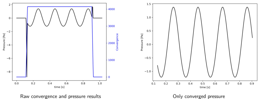
antares.utils.FWH.extract_converged_signal(base, subtract_mean=False, start_at_zero=False)

Extract the converged part of a FWH result base.

The converged signal corresponds to the part of the signal where the convergence variable is at its maximum. An additional check if performed to ensure that this converged region corresponds to a continuous temporal signal. A warning is printed otherwise.

The output base contains as many zones as observers. Each zone contains one instant. The instant contains the converged time vector and the converged pressure variables.

Additionally, the pressure signals can be shifted by subtracting its mean. And the vector time can be shifted so it always starts at zero for each observer.

Parameters:

• base (Base) – The base containing the FWH results

• subtract_mean (bool) – True if should subtract the mean value for each contribution.

• start_at_zero (bool) – True if should shift the observers time vectors so they all start at zero.

Returns:

An antares Base with the converged signals

import antares
from antares.utils.FWH import extract_converged_signal

reader = antares.Reader('hdf_antares')
reader['filename'] = 'my_fwh_results.h5'
base = reader.read()

converged_results = extract_converged_signal(base, subtract_mean=False, start_at_zero=False)

Find signal periodicity

antares.utils.FWH.find_periodicity(base, equal_for_all_obs=False)

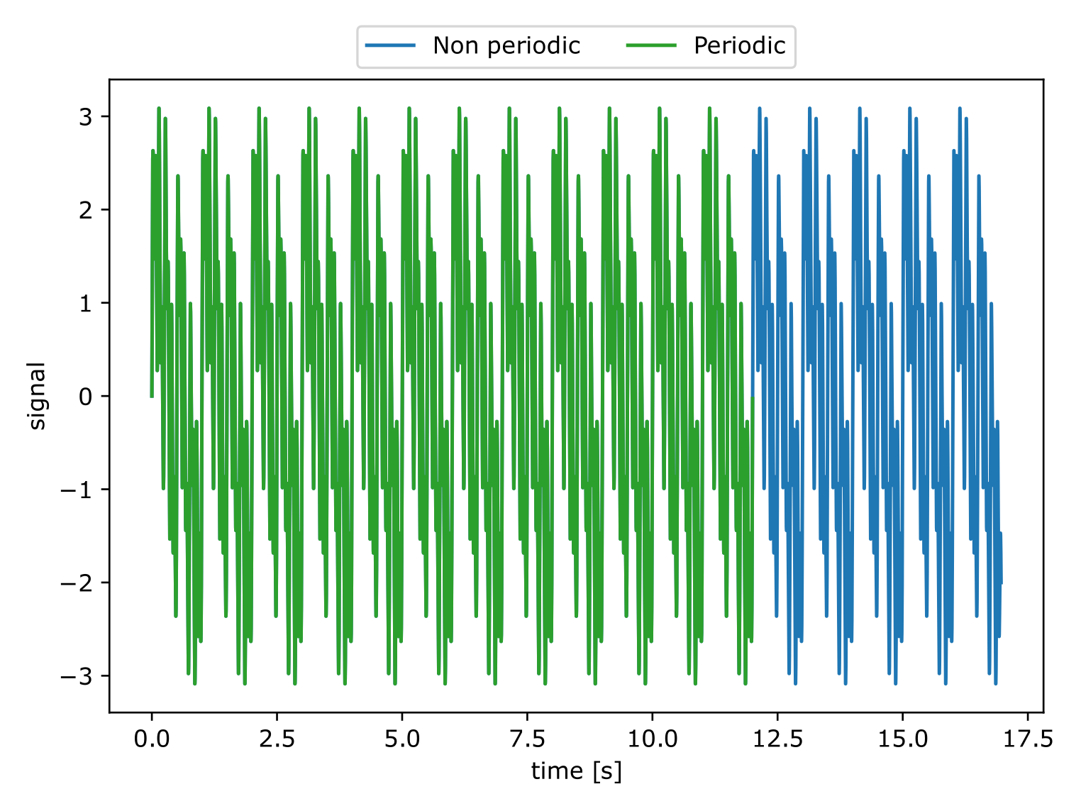
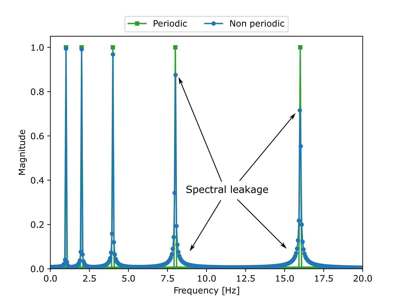
Cut the observer signal to make it as periodic as possible.

This helps to reduce the spectral leakage when doing the FFT Treatment.

The cutting point is defined as the point where the cross-correlation between the first and second halves of the cut signal is maximum.

Parameters:

• base (Base) – The base containing converged FWH results

• equal_for_all_obs (bool) – True if the cutting point is the same for all observers, this will reduce computational time

Returns:

An antares Base with the same format as the input base, but with the signal cut for all observers.

Usage:

import antares
from antares.utils.FWH import find_periodicity

reader = antares.Reader('hdf_antares')
reader['filename'] = 'fwh_results.h5'
base = reader.read()

periodic_base = find_periodicity(base, equal_for_all_obs=False)

The following example illustrates the effects of the spectral leakage when a FFT is performed on a non perfectly periodic signal. The signal corresponds to the function:

\[y(t) = sin(2\pi t) + sin(4\pi t) + sin(8 \pi t) + sin(16 \pi t) + sin(32 \pi t)\]

This signal has a period \(T=2 \pi\) but it was sampled from \([0, 5.5 \pi]\) which does not correspond to an integer multiple of \(T\). We remark that doing a Fourier transform over such signal leads to wrong amplitude values as well as parasitic noise. The function antares.utils.FWH.find_signal_periodicty cuts the signal at the right place to have a perfectly periodic signal. The FFT of such signal is exactly 5 peaks at the right frequencies and with the correct magnitude.

Add FWH results

antares.utils.FWH.add_fwh_results(bases, rtol=1e-05, atol=1e-08)

Add the pressure signal (and contributions) of different FWH result bases into one single base.

Parameters:

• bases (list(Base)) – list of bases containing different fwh results.

• rtol (float) – The relative tolerance parameter, 1e-05 by default as in numpy

• atol (float) – The absolute tolerance parameter, 1e-08 by default as in numpy

Returns:

A base with the same format as the FWH result base but with the pressure signal added for each observer.

Warning

The time discretizations for all input bases are assumed to be identical.

Usage:

import antares
from antares.utils.FWH import add_fwh_results

reader1 = antares.Reader('hdf_antares')
reader1['filename'] = 'fwh_surface_1.h5'
surface1 = reader1.read()

reader2 = antares.Reader('hdf_antares')
reader2['filename'] = 'fwh_surface_2.h5'
surface2 = reader2.read()

total_results = add_fwh_results([surface1, surface2])

Print Attributes

antares.utils.FWH.print_fwh_attributes(base)

Print base level attributes of FWH result bases in a pretty format.

The attributes are split into 4 different categories:

• Treatment keywords.

• Git information.

• System information.

• Miscellaneous information.

The attributes of each category are printed in alphabetical order (case insensitive).

Parameters:

base (Either Base or a str with the path for the base.) – The base containing the FWH results.

Normal vectors helper functions

The module antares.utils.FWH contains several helper functions that implement the most common scenarios to compute the normal vectors:

Compute normal vectors using mesh topology

antares.utils.FWH.compute_normals_from_topology(invert=False)

Compute the normal vectors using the connectivity list of the mesh.

If the connectivity list is correctly ordered, the normal vectors computed from the connectivity will all by oriented in the same way (either inwards or outwards).

Parameters:

invert (bool) – False if the normal should be computed using the order in the connectivity list. True if they should be inverted.

Usage:

import antares
from antares.utils.FWH import compute_normals_from_topology

treatment = antares.Treatment('fwh')
treatment['compute_normal_vectors'] = compute_normals_from_topology(invert=False)
# .
# .
# .
treatment.execute()

Compute normal vectors and auto-orient them

antares.utils.FWH.compute_normals_auto_orient(orientation=1, extra_params={})

Compute the normal vectors using the treatment ‘cellnormal’ and tries to auto-orient them in the same direction using the ‘auto_orient’ parameter.

The orientation can be changed using the orientation parameter and extra parameters can be passed to the treatment using the extra_params argument.

The limitations of this function are the same limitations as the ‘auto_orient’ feature in the ‘cellnormal’ treatment.

Parameters:

• orientation (int) – The orientation parameter for the ‘cellnormal’ treatment.

• extra_params (dict) – Any other parameter that should be passed to the ‘cellnormal’ treatment.

Usage:

import antares
from antares.utils.FWH import compute_normals_auto_orient

treatment = antares.Treatment('fwh')
treatment['compute_normal_vectors'] = compute_normals_auto_orient(orientation=1, extra_params={})
# .
# .
# .
treatment.execute()

Compute normal vectors and orient them using a reference point

antares.utils.FWH.compute_normals_orient_using_point(ref_point)

Compute the normal vectors and orient them so all the vectors are pointing away from a reference point.

Parameters:

ref_point (list(float)) – The reference point

Usage:

import antares
from antares.utils.FWH import compute_normals_orient_using_point

treatment = antares.Treatment('fwh')

# all normal vectors will point away from the origin ([0, 0, 0])
treatment['compute_normal_vectors'] = compute_normals_orient_using_point([0, 0, 0])
# .
# .
# .
treatment.execute()

Modify surface and volume databases helper functions

antares.utils.FWH.keep_nodes(variables, thresholds)

Modify the FWH database keeping only the nodes that respect a given threshold for a given list of variables.

Parameters:

• variables (list(str)) – List of variables to which apply the threshold

• thresholds – List of tuples containing the lower and upper limit for the threshold. If either the lower or upper limit is None, the threshold will not be applied to that limit.

Usage:

import antares
from antares.utils.FWH import keep_nodes

treatment = antares.Treatment('fwh')

# Keep all nodes with a pressure less than 1e15 and with a density between 0 and 1e15
treatment['modify_surface'] = keep_nodes(['pressure', 'density'], [(None, 1e15), (0, 1e15)])
# .
# .
# .
treatment.execute()

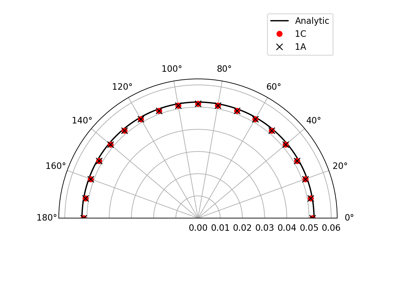
Validation

This treatment was validated using a serie of academic test cases for which the theoretical solution can be derived. These test cases can be found in the papers of Casalino (2003) and Najafi-Yazdi et al. (2011):

• Static monopole, dipole or quadrupole in a static or moving medium.

• Rotating monopole in a static or moving medium.

• Rotating dipole in a static medium.

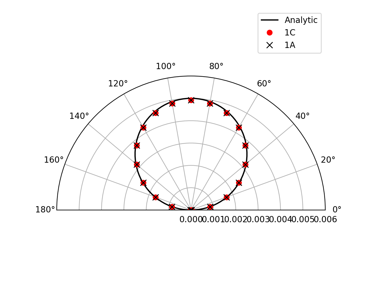
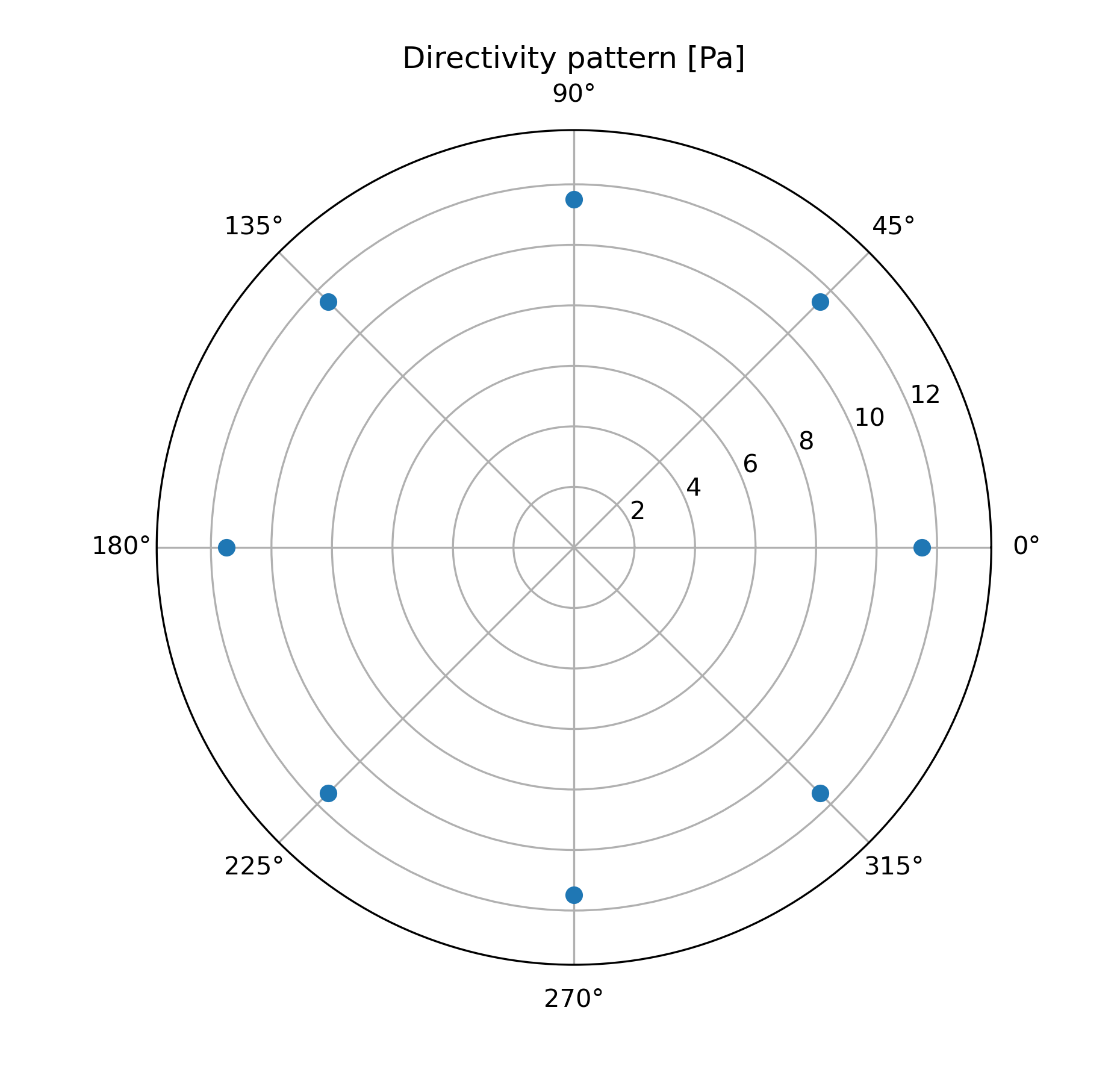
Below, we can find a few results of these test cases:

• Farfield directivity pattern (rms pressure) of a static point monopole (left) and a point dipole (right) measured at \(r=40l\), radiating in a medium at rest (M=0):

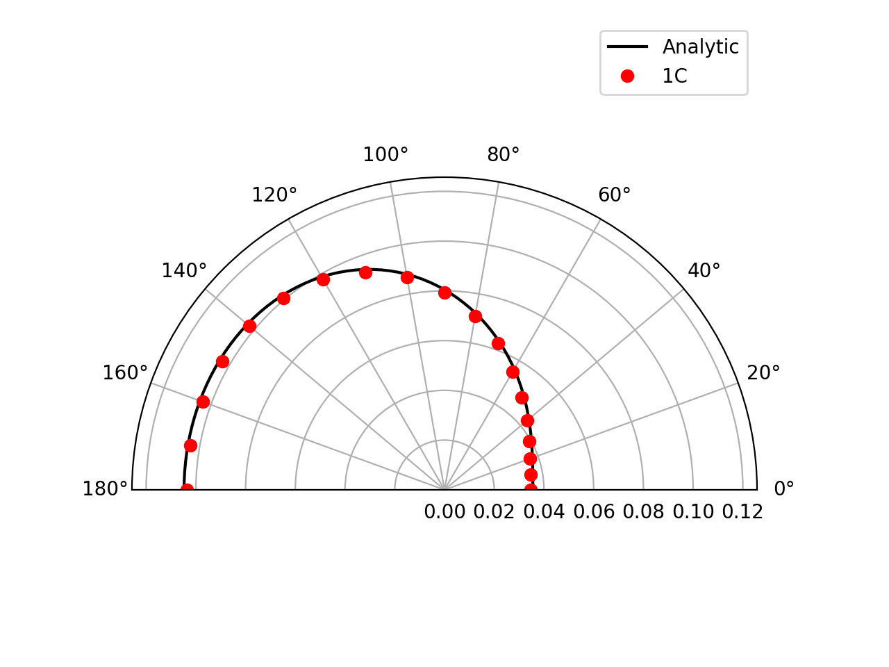
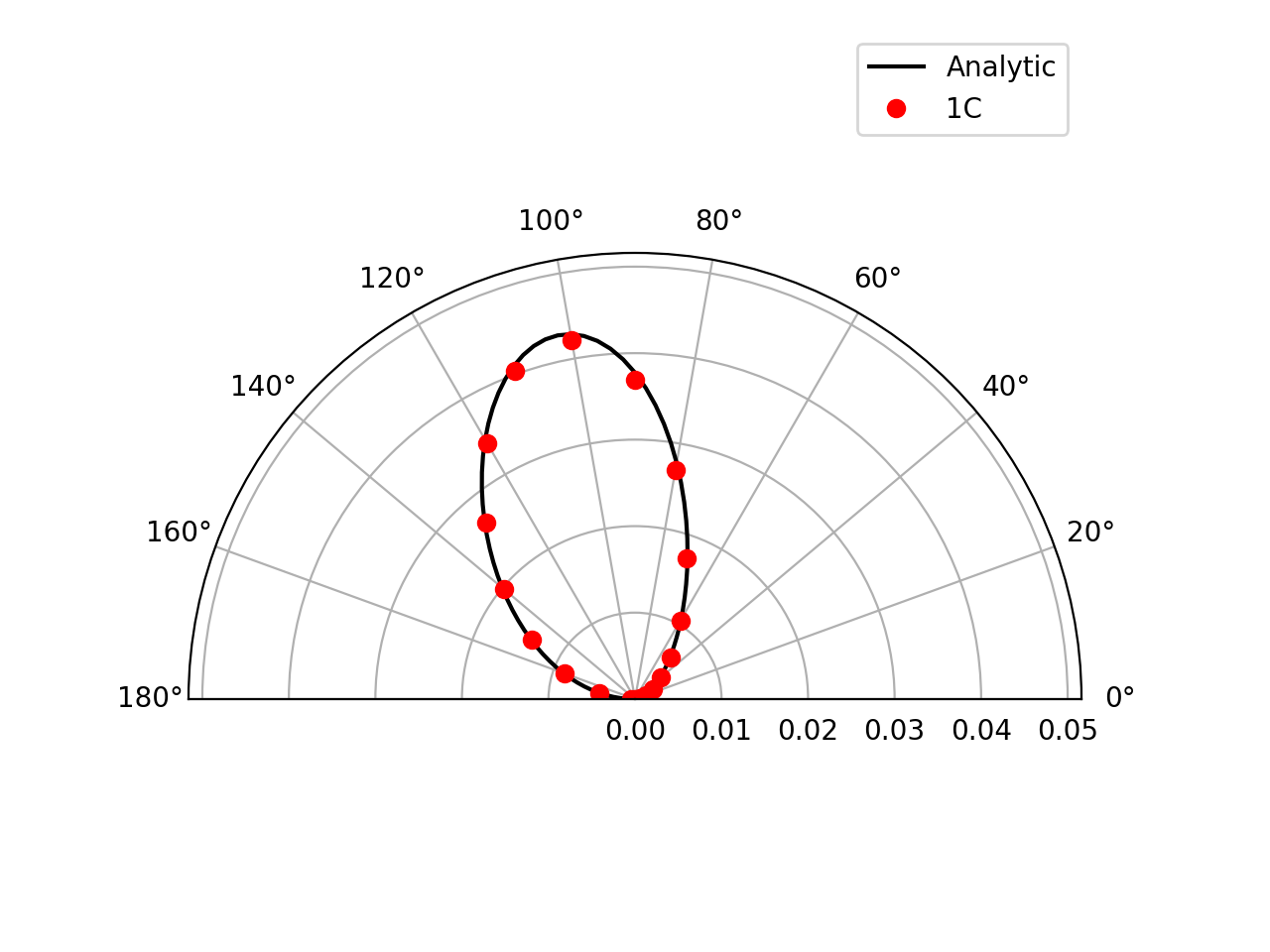
• Farfield directivity pattern (rms pressure) of a static point monopole (left) in a flow at M=0.5 and a point dipole (right) in a flow at M=0.8, measured at \(r=40l\)

Examples

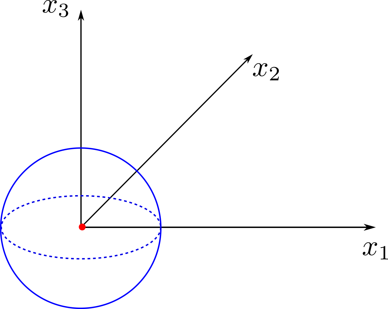
Example 1: Acoustic directivity of a static monopole

The following example shows the setup to compute the acoustic field using a static mesh. The test case corresponds to a single monopole located at the origin. The chosen FWH surface is a sphere of 50cm diameter centered at the monopole position. A scheme and an example of the generated database is presented below:

The treatment script can be found in antares/examples/treatment/fwh_mono.py and the post-treatment script: antares/examples/treatment/post_fwh_mono.py

"""
Ffowcs Williams & Hawkings Analogy

In parallel: mpirun -np NPROCS python fwh_mono.py
In serial: python fwh_mono.py
"""
import os
if not os.path.isdir('OUTPUT'):
    os.makedirs('OUTPUT')

import antares
from antares.utils.FWH import compute_normals_from_topology



# Read base
r = antares.Reader('bin_tp')
r['filename'] = os.path.join('..', 'data', 'FWH', 'Monopole', 'monopole_<instant>.plt')
base = r.read()

# Apply FWH treatment
treatment = antares.Treatment('fwh')
treatment['base'] = base
treatment['analogy'] = '1A'
treatment['type'] = 'porous'
treatment['compute_normal_vectors'] = compute_normals_from_topology()
treatment['obs_file'] = os.path.join('..', 'data', 'FWH', 'fwhobservers_monopole.dat')
treatment['pref'] = 97640.7142857
treatment['tref'] = 287.6471952408
treatment['dt'] = 0.00666666666667
treatment['output'] = os.path.join('OUTPUT', "fwh_result")
fwhbase = treatment.execute()

Post-treatment example: The directivity pattern

The following script shows an example of how to compute the directivity pattern in the \(x_1-x_2\) plane

"""

Post-Treatment script for a FW-H solver output database

input: FW-H database
output: raw signal, RMS, SPL, OASPL

"""

# -------------------------------------------------------------- #
# Import modules
# -------------------------------------------------------------- #

import os
if not os.path.isdir('OUTPUT'):
    os.makedirs('OUTPUT')

import numpy as np
import matplotlib.pyplot as plt
from antares import *
from antares.utils.Signal import *


# -------------------------------------------------------------- #
# Input parameters
# -------------------------------------------------------------- #

# Input path
IN_PATH = 'OUTPUT' + os.sep
INPUT_FILE = ['fwh_result.h5']
# Can sum different surface if needed, then give a list
# INPUT_FILE = ['surface1.h5', 'surface2.h5', 'surface3.h5']

# Output path
OUT_PATH = 'OUTPUT' + os.sep
# output name extension
NAME = 'FWH_'
# output name extension
EXT = 'CLOSED'

# Azimuthal Average
AZIM = False

# Convert in dB
LOG_OUT = False

# Keep the largest convective time (azimuthal mean should not work)
MAX_CONV = False

# Extract converged pressure signal in separate files
RAW = False

# Extract R.M.S from raw pressure fluctuation (only if AZIM=False)
RMS = False

# Compute Third-Octave
ThirdOctave = False

# PSD parameter
PSD_Block = 1
PSD_Overlap = 0.6
PSD_Pad = 1

# smoothing filter for psd (Only for a broadband noise)
Smooth = False
# 1: mean around a frequency, 2: convolution
type_smooth = 1
# percent of frequency to filter
alpha = 0.08

# filter initial signal (if frequency = -1.0 no filtering)
Filter = False
Lowfreq = -1.0
Highfreq = -1.0

# downsampling signal if necessary
downsampling = False
# 1: order 8 Chebyshev type I filter, 2: fourier method filter, 3: Gaussian 3 points filter
type_down = 3
# downsampling factor
step = 3

# frequency to keep for OASPL (if not all, give a range [100, 1000] Hz)
FREQ_RANGE = 'all'

# Observers informations
# number of obs. in azimuthal direction
NB_AZIM = 1
# Angle between two microphone in  the streamwise direction
dTH = 45.
# Minimum and maximum angle of observers in the streamwise direction
a_min = 0.0
a_max = 315.0
# observers
observers = np.arange(a_min, a_max+dTH, dTH)
nb_observer = len(observers)*NB_AZIM

# -------------------------------------------------------------- #
# Script template
# -------------------------------------------------------------- #

print(' \n>>> -----------------------------------------------')
print(' >>>        Post-processing of FW-H results')
print(' >>> -----------------------------------------------')

nbfile = len(INPUT_FILE)
PSD = [PSD_Block, PSD_Overlap, PSD_Pad]
FILTER = [Filter, Lowfreq, Highfreq, Smooth, type_smooth, alpha, downsampling, type_down, step]
obs_info = [nb_observer, NB_AZIM, dTH, observers]
outfile = [OUT_PATH, NAME, EXT]

spl_datafile, oaspl_datafile, oaspl_raw_datafile, raw_datafile = build_outputfile_name(outfile, FILTER, AZIM, LOG_OUT)

if nbfile == 1:
    r = Reader('hdf_antares')
    r['filename'] = IN_PATH+INPUT_FILE[0]
    base = r.read()
else:
    r = Reader('hdf_antares')
    r['filename'] = IN_PATH+INPUT_FILE[0]
    base = r.read()
    for file in INPUT_FILE[1:]:

        r = Reader('hdf_antares')
        r['filename'] = IN_PATH+file
        base2add = r.read()

        # Sum signal
        #  + CONV=True: only the common converged part of each surfaces is keep
        #  + CONV=False: Keep all the converged part
        base = AddBase2(base, base2add, CONV=True)

# Keep only converged signal
#   + if MAX_CONV = False the signal will be truncated to the common converged part between each observers
base, observers_name = prepare_data(base, obs_info, MAX_CONV=True)

# Compute SPL and OASPL
# OUT_BASE
SPL, OASPL, OASPL_RAW, RAW, SPL_BAND = compute_FWH(base, obs_info, PSD, FILTER,
                                                   MAX_CONV, LOG_OUT,
                                                   FREQ_RANGE,
                                                   RAW_DATA=RAW,
                                                   AZIMUTHAL_MEAN=AZIM,
                                                   CHECK_RMS=RMS,
                                                   BAND=ThirdOctave)

# Checking if the output_path exists
OUT_PATH = '.' + os.sep
if not os.path.exists(OUT_PATH):
    os.makedirs(OUT_PATH)

# write result
w = Writer('column')
w['base'] = SPL
w['filename'] = spl_datafile
w.dump()

w = Writer('column')
w['base'] = OASPL
w['filename'] = oaspl_datafile
w.dump()

if OASPL_RAW is not None:
    w = Writer('column')
    w['base'] = OASPL_RAW
    w['filename'] = oaspl_raw_datafile
    w.dump()

if RAW is not None:
    w = Writer('column')
    w['base'] = RAW
    w['filename'] = raw_datafile
    w.dump()

if SPL_BAND is not None:
    index = spl_datafile.find('.dat')
    spl_third_octave = spl_datafile[:index] + '_third_octave' + spl_datafile[index:]
    w = Writer('column')
    w['base'] = SPL_BAND
    w['filename'] = spl_third_octave
    w.dump()



## Plot directivity pattern
fig = plt.figure(figsize=(6.2,6))
ax = fig.add_subplot(111, polar=True)
theta_plot = OASPL[0][0][0]*np.pi/180
p_rms = (OASPL[0][0][1])**0.5

plt.title('Directivity pattern [Pa]')
ax.plot(theta_plot, p_rms, marker='o', linestyle='')
ax.set_rmax(p_rms.max()*1.2)
plt.savefig(os.path.join('.', 'OUTPUT', 'directivity.png'), dpi=300)

Example 2: Pressure signal of a rotating monopole

The treatment script can be found in antares/examples/treatment/fwh_rotating_reference_frame.py and the post-treatment script: antares/examples/treatment/post_fwh_rotating_reference_frame.py

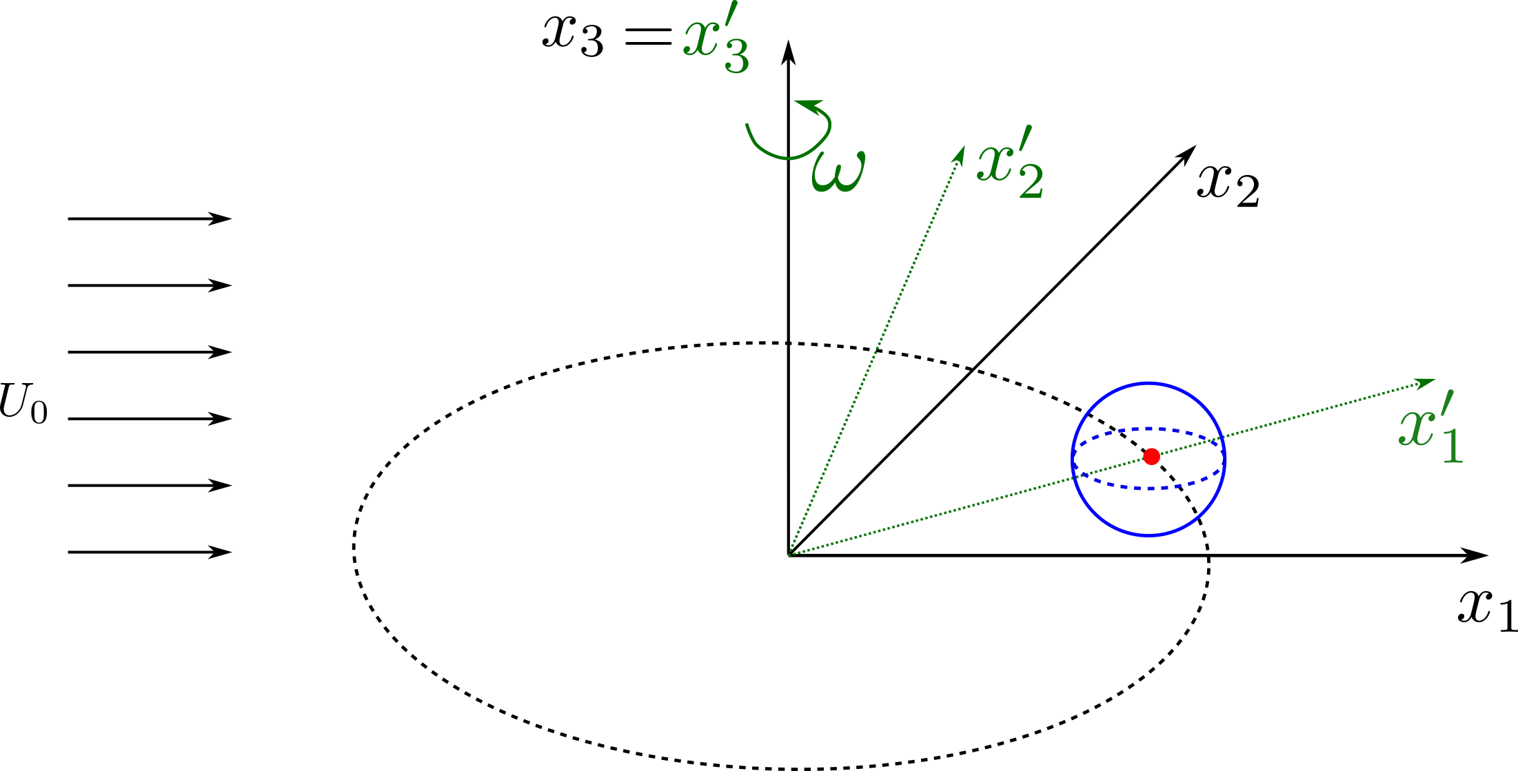
The following example shows how to setup a case with a mesh in a rotating reference frame. The test case is a single acoustic monopole rotating around the axis \(x_3\) with an angular velocity equals to \(2\pi \frac{rad}{s}\). There is a absolute mean flow (\(M=0.5\)) in the \(x_1\) direction. There are two different frame of references: \(x_1-x_2-x_3\) is the absolute static frame of reference and \(x_1^{\prime}-x_2^{\prime}-x_3^{\prime}\) is frame of reference rotating with the monopole. All the quantities of the FWH surface are computed with respect to this rotating frame of reference. The figures below show a schematic representation of the test case and an example of the database

The script to study this case is as follow:

import antares
import os
import numpy as np
from antares.utils.FWH import compute_normals_orient_using_point

if not os.path.isdir('OUTPUT'):
    os.makedirs('OUTPUT')

## Read base
reader = antares.Reader('bin_tp')
reader['filename'] = os.path.join('..', 'data', 'FWH', 'Rotating_monopole', 'rotating-monopole-x1x2_<instant>.plt')
base = reader.read()

# Apply FWH treatment
treatment = antares.Treatment('fwh')
treatment['base'] = base
treatment['analogy'] = '1C'
treatment['type'] = 'porous'
treatment['obs_file'] = os.path.join('..', 'data', 'FWH', 'Rotating_monopole', 'fwhobservers.dat')
treatment['mach'] = 0.5
treatment['pref'] = 97640.71428571429
treatment['tref'] = 287.6471952407826
treatment['dt'] = 0.005025125628140704
treatment['compute_normal_vectors'] = compute_normals_orient_using_point([1, 0, 0])
treatment['rotation_velocity'] = 2*np.pi*1.0
treatment['rotation_axis'] = [0, 0, 1]
treatment['mesh_kinetics'] = 'rotating_reference_frame'
treatment['pressure_variable'] = 'p'
treatment['density_variable'] = 'rho'
treatment['velocity_variables'] = ['u', 'v', 'w']
treatment['output'] = os.path.join('OUTPUT', 'rotating_monopole')
treatment.execute()

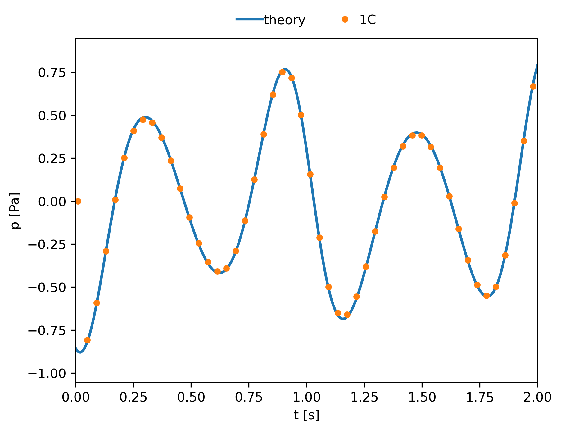
Post-Treatment example: The signal pressure for a single observer

We can compare the analytical solution with the solution obtained with the treatment using the following script:

import antares
import os
import matplotlib.pyplot as plt
import numpy as np


## Read theoretical pressure and time vectors
theoretical_filename = os.path.join('..', 'data', 'FWH', 'Rotating_monopole', 'analytical_pressure.dat')
theoretical_reader = antares.Reader('column')
theoretical_reader['filename'] = theoretical_filename
theoretical_base = theoretical_reader.read()
theoretical_time = theoretical_base[0][0]['time']
theoretical_p = theoretical_base[0][0]['pressure1']

## Read antares pressure and time vectors
ant_filename = os.path.join('OUTPUT', 'rotating_monopole.h5')
ant_reader = antares.Reader("hdf_antares")
ant_reader['filename'] = ant_filename
ant_base = ant_reader.read()
ant_time = ant_base[0][0]['time']
ant_pressure = ant_base['obs_1'][0]['pressure']

# plt.figure(figsize=(6.2,4.65)) 

## Plot 1C results
plt.plot(theoretical_time, theoretical_p, linewidth=2, label='theory')
plt.plot(ant_time, ant_pressure, marker='o', linestyle='',
         markevery=4, label='1C', markersize=4)

## Add labels, legends and other configurations
plt.xlim([0, np.max(theoretical_time)])
plt.ylim([1.2*np.min(theoretical_p), 1.2*np.max(theoretical_p)])
plt.xlabel('t [s]')
plt.ylabel('p [Pa]')
plt.legend(ncol=3,  loc='lower center', bbox_to_anchor=(0.5, 1.0),
           handletextpad=0.1, labelspacing=0, frameon=False)

## Save plot
output = os.path.join('OUTPUT', 'plot.png')
plt.savefig(output, bbox_inches='tight', dpi=300)
plt.close()

FAQ

Datafile vs base keywords

The input database can be specified by using either the base keywords or datafile (with the optional meshfile) keyword. The latter only works when the base is written such as every instant is stored in a different file (i.e. using the <instant> tag). In this case, each instant file is read independently and not as part of a whole database. This is a more efficient reading strategy as only 2-3 instants are only ever fully loaded into memory. This could be more efficient than feeding the whole database through the base keywords as, depending on each reader, the lazy loading of variables or the shared mesh feature might not be available.

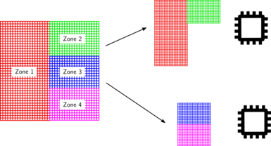
How does the treatment split the database when using MPI?

The splitting of the input database in the different processors of an MPI run depends on the number of zones present in the database:

1. If the input database contains only one zone, the database is split by distributing as equally as possible the cells into the total number of processors. This ensures that workload is well balanced between all processors. It also ensure that we can use as many processors as cell there are in the database.

2. If the input database contains 2 or more zones, the database is split by distributing as equally as possible the zones into the total number of processors. This does not ensure that the workload is well balanced between all processors; as different zones could contain different numbers of cells. This also limits the number of active processors the treatment will use, because it will never be greater than the number of zones. If you have a small number of zones and you want to use a large number of processors, a merge treatment must be performed before using the FWH treatment.

In which order are the equation variables computed?

The order in which the equations for the physical variables are computed is the following:

1. Pressure.

2. Density.

3. Velocity in \(x\) direction.

4. Velocity in \(y\) direction.

5. Velocity in \(z\) direction.

References

Casalino, D. (2003). An advanced time approach for acoustic analogy predictions. Journal of Sound and Vibration, 261(4), 583-612. (link).

Shur, M. L., Spalart, P. R., & Strelets, M. K. (2005). Noise prediction for increasingly complex jets. International journal of aeroacoustics, 4(3), 213-245. (part 1, part 2)

Farassat, F. (2007). Derivation of Formulations 1 and 1A of Farassat. Nasa/TM-2007-214853, p. 1–25.(link).

Morfey, C. L., & Wright, M. C. M. (2007). Extensions of Lighthill’s acoustic analogy with application to computational aeroacoustics. Proceedings of the Royal Society A: Mathematical, Physical and Engineering Sciences, 463(2085), 2101-2127. (link)

Spalart, P. R., & Shur, M. L. (2009). Variants of the Ffowcs Williams-Hawkings equation and their coupling with simulations of hot jets. International journal of aeroacoustics, 8(5), 477-491. (link).

Najafi-Yazdi, A., Brès, G. A., & Mongeau, L. (2011). An acoustic analogy formulation for moving sources in uniformly moving media. Proceedings of the Royal Society A: Mathematical, Physical and Engineering Sciences, 467(2125), 144-165. (link).

Rahier, G., Huet, M., & Prieur, J. (2015). Additional terms for the use of Ffowcs Williams and Hawkings surface integrals in turbulent flows. Computers & Fluids, 120, 158-172. (link)

Ikeda, T., Enomoto, S., Yamamoto, K., & Amemiya, K. (2017). Quadrupole corrections for the permeable-surface Ffowcs Williams–Hawkings equation. AIAA Journal, 55(7), 2307-2320. (link)