
Chorochronic Reconstruction (Synchronous)
Description
Compute the chorochronic (or multi-chorochronic) reconstruction of a CFD computation for synchronous phenomenon.
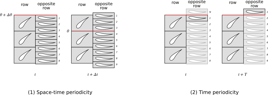
In turbomachinery, a chorochronic simulation takes into account two types of periodicity of the flow:
a space-time periodicity, when rows return back to the same relative position of rows shifted of a number of blades.
a time periodicity, when rows return back to the same relative position with no shift.
Formally, for scalar fields, those periodicies are expressed as follows:
\(w(\theta + \Delta \theta, t) \; = \; w(\theta, t + \Delta t)\),
\(w(\theta, t + T) \; = \; w(\theta, t)\).
For vector fields in cartesian coordinates, those expressions are:
\(\vec{w}(\theta + \Delta \theta, t) \; = \; \text{rot}_{\Delta \theta} \cdot \vec{w}(\theta, t + \Delta t)\),
\(\vec{w}(\theta, t + T) \; = \; \vec{w}(\theta, t)\).
The these relations, \(\theta\) is the azimuth in the rotating frame of the current row.
The azimuthal continuity of the flow (\(2 \pi\) periodicity) can be retrieved from those relations (see Formulae).
The reconstruction is based on Discrete Fourier Transform that simplifies chorochronic condition 1. The treatment is based on instant numbers and time iterations instead of real time. For theoretical details, see Formulae.
The data is given on a grid in relative cartesian coordinates (unmoving mesh). The reconstructed data is put a a grid in absolute cartesian coordinates, that can move for rows that have a nonzero rotation speed. In particular, after reconstruction, vectors (assumed expressed in cartesian coordinates) are additionally rotated.
Construction
import antares
myt = antares.Treatment('chororeconstruct')
Parameters
- base:
Base The input base that will be chorochronically duplicated.
- base:
- type: str, default= ‘fourier’
The type of approach (‘fourier’ or ‘least_squares’) used to determine the amplitudes and phases of each interaction mode. If ‘fourier’, a DFT is performed: in the case of a single opposite row, the base should contain enough instants to cover the associated pattern of blades passage (‘nb_ite_rot’ / ‘extracts_step’ * ‘nb_blade_opp_sim’/ ‘nb_blade_opp’); in the case of multiple opposite rows, the base should contain enough instants to cover a complete rotation (‘nb_ite_rot’ / ‘extracts_step’). If ‘least_squares’, a least-squares approach is used. For robustness and accuracy reasons, it is advised to have enough instants in the base to cover at least two blade passages (2 * ‘nb_ite_rot’ / ‘extracts_step’ / ‘nb_blade_opp’).
- coordinates: list(str)
The variable names that define the set of coordinates used for duplication. It is assumed that these are in cartesian coordinates.
- vectors: list(tuple(str), default= []
If the base contains vectors, these must be rotated. It is assumed that they are expressed in cartesian coordinates.
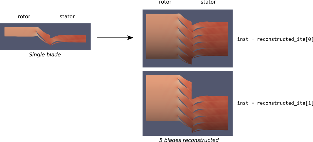
- reconstructed_ite: list(int), default= [0]
List of iterations to be reconstructed.
- nb_blade: int or ‘in_attr’, default= ‘in_attr’
Number of blades of the current row. If ‘in_attr’, then each zone of the base must have an attribute ‘nb_blade’.
- nb_blade_sim: int or ‘in_attr’, default= 1
Number of blades simulated of the current row. If ‘in_attr’, then each zone of the base must have an attribute ‘nb_blade_sim’.
- nb_blade_opp: int or list(int) or ‘in_attr’, default= ‘in_attr’
Number of blades of the opposite row (or list of numbers of blades of the opposite rows in the case of multiple opposite rows). If ‘in_attr’, then each zone of the base must have an attribute ‘nb_blade_opp’.
- nb_blade_opp_sim: int or list(int) or ‘in_attr’, default= ‘in_attr’
Number of blades simulated of the opposite row (or list of numbers of blades simulated of the opposite rows in the case of multiple opposite rows). If ‘in_attr’, then each zone of the base must have an attribute ‘nb_blade_opp_sim’.
- omega: float or ‘in_attr’, default= ‘in_attr’
Rotation speed of the current row expressed in radians per second. If ‘in_attr’, then each zone of the base must have an attribute ‘omega’.
- omega_opp: float or list(float) or ‘in_attr’, default= ‘in_attr’
Rotation speed of the opposite row (or list of rotation speeds of the opposite rows in the case of multiple opposite rows) expressed in radians per second. If ‘in_attr’, then each zone of the base must have an attribute ‘omega_opp’.
- nb_harm: int or ‘in_attr’, default= None
Number of harmonics used for the reconstruction. If it is not given, all the harmonics are computed for type ‘fourier’ and the first three harmonics are computed for type ‘least_squares’. If ‘in_attr’, then each zone of the base must have an attribute ‘nb_harm.
- nb_ite_rot: int
The number of time iterations to describe a complete rotation, i.e. the period in number of iterations for which rows get back to the same relative position (e.g. if blade 1 of row 1 is in front of blade 3 of row 2, then it is the period in number of iterations to get back to the same configuration).
- extracts_step: int, default= 1
The number of time iterations between two instants of the base. This number is assumed constant over pairs of successive instants.
- nb_duplication: int or tuple(int) or ‘in_attr’, default= ‘in_attr’
Number of duplications if an integer is given (given base included). Range of duplications if a tuple is given (from first element to second element included). If ‘in_attr’, then each zone of the base must have an attribute ‘nb_duplication’.
- ite_init: int, default= 0
Iteration of the first instant of the base.
- recompute_theta: bool , default = False
If True, the treatment will recompute the cylindrical theta coordinate using the ComputeCylindrical treatment
- axis: list(float), default = None
The axis of the cylindrical coordinate system. If None it will use the default of the ComputeCylindrical treatment
- origin: list(float), default = [0.0, 0.0, 0.0]
The origin of the cylindrical coordinate system
Preconditions
The coordinates of each row must be given in the relative (rotating) frame, i.e. constant over instants.
In case of a single opposite row, there must be enough instants to cover a time period \(T\).
In case of multiple opposite rows, there must be enough instants to cover a complete rotation, i.e. the period for which rows get back to the same relative position.
As the treatment is based of Discrete Fourier Transform on the time variable, there must be enough instants to fulfill hypotheses of the Nyquist-Shannon sampling theorem.
Vectors and coordinates must be given in cartesian coordinates.
Postconditions
The output base contains for each row nb_duplication times more zones than the input base.
The output base is given in the absolute (fixed) frame, i.e. moving mesh over instants.
Warnings
If you use an equation manager which assumes that some quantities are constant (for instance the adiabatic index gamma and the ideal gas constant R in equation manager “internal”) and if you compute new variables (for instance entropy s) BEFORE the reconstruction: After the reconstruction, you should delete those constants quantities and compute them again. If not, the value of those such constant quantities are reconstructed and thus are approximated.
Academic example
"""
Example of two rows chorochronic reconstruction of an academic case.

Let us consider the following two rows machine:
- Rotor: 25 blades, at 22000 rad/s.
- Stator: 13 blades, at 0 rad/s.

The flow is described by the following field v, fulfilling both periodicities:
(1) v(theta + DTHETA, t) = v(theta, t + DT)
(2) v(theta, t + T) = v(theta, t)
where DTHETA is the pitch of the rotor, DT is the chorochronic period, and T
is the opposite row blade passage period,
    v(theta, t) = cos(5.0*r)* sin((NB_BLADE_OPP - NB_BLADE)
                                  *(theta + t*DTHETA/DT))

Let us consider an axial cut of one sector (one blade) of the rotor of this
machine.
This code shows how to reconstruct 9 blades over 30 iterations of
one stator blade passage.
"""
import os

import numpy as np
import antares

OUTPUT = 'OUTPUT'
if not os.path.isdir(OUTPUT):
    os.makedirs(OUTPUT)

# properties of the machine
NB_BLADE = 25
NB_BLADE_OPP = 13
OMEGA = 22000.0
OMEGA_OPP = 0.0

# chorochronic properties of the machine
DTHETA = 2.0*np.pi/NB_BLADE
DT = 2.0*np.pi*(1.0/NB_BLADE_OPP - 1.0/NB_BLADE)/(OMEGA_OPP - OMEGA)
T = 2.0*np.pi/NB_BLADE_OPP/abs(OMEGA_OPP - OMEGA)

# properties of discretization
N_THETA = 50
N_R = 50
EXTRACTS_STEP = 1
TIMESTEP = 1.0e-7

# number of instants to cover the time period T
NB_INST_ALL_POSITIONS = int(np.ceil(T/TIMESTEP/EXTRACTS_STEP))

# build the sector
b = antares.Base()
b['rotor_xcut'] = antares.Zone()
r = np.linspace(1.0, 2.0, N_R)
theta = np.linspace(0.0, DTHETA, N_THETA)
r, theta = np.meshgrid(r, theta)
b[0].shared['x'] = np.zeros_like(r)
b[0].shared['r'] = r
b[0].shared['theta'] = theta
b.compute('y = r*cos(theta)')
b.compute('z = r*sin(theta)')
del b[0].shared['r']
del b[0].shared['theta']
for idx_inst in range(NB_INST_ALL_POSITIONS):
    inst_key = str(idx_inst)
    b[0][inst_key] = antares.Instant()
    t = TIMESTEP*EXTRACTS_STEP*idx_inst
    b[0][inst_key]['v'] = np.cos(5.0*r) * np.sin((NB_BLADE_OPP - NB_BLADE)
                                                 *(theta + t*DTHETA/DT))

# number of iterations to perform a complete rotation of the opposite
# row relatively to the current row
NB_ITE_ROT = 2.0*np.pi/abs(OMEGA_OPP - OMEGA)/TIMESTEP

# perform chorochronic reconstruction on one blade passage
ITE_BEG = 0
ITE_END = T/TIMESTEP
ITE_TO_RECONSTRUCT = np.linspace(ITE_BEG, ITE_END, 30)
t = antares.Treatment('chororeconstruct')
t['base'] = b
t['type'] = 'fourier'
t['coordinates'] = ['x', 'y', 'z']
t['vectors'] = []
t['reconstructed_ite'] = ITE_TO_RECONSTRUCT # covers one blade passage
t['nb_blade'] = NB_BLADE
t['nb_blade_sim'] = 1
t['nb_blade_opp'] = NB_BLADE_OPP
t['nb_blade_opp_sim'] = 1
t['omega'] = OMEGA
t['omega_opp'] = OMEGA_OPP
t['nb_harm'] = None
t['nb_ite_rot'] = NB_ITE_ROT
t['extracts_step'] = EXTRACTS_STEP
t['nb_duplication'] = 9 # to get 9 blades
t['ite_init'] = 0
b_choro = t.execute()

# write the result
w = antares.Writer('hdf_antares')
w['base'] = b_choro
w['filename'] = os.path.join(OUTPUT, 'ex_choro_academic')
w.dump()
Real-case example
"""
Example for the treatment chororeconstruct

This test case is CPU intensive
"""
import antares
from math import pi
import os
if not os.path.isdir('OUTPUT'):
    os.makedirs('OUTPUT')

results_directory = os.path.join("OUTPUT", 'ex_CHORO_RECONSTRUCTION')
if not os.path.exists(results_directory):
    os.makedirs(results_directory)

# Chorochronic properties
N_front = 30  # number of blades of front row
N_rear  = 40  # number of blades of rear row
nb_duplication_front = N_front  # number of duplications for front row (can be different from the number of blades)
nb_duplication_rear = N_rear  # number of duplications for rear row (can be different from the number of blades)

nb_ite_per_rot = 9000  # number of iterations per rotation
extracts_step = 5  # extraction step

omega_front = -1.947573300000e-03  # speed of rotation of front row (rad/s)
omega_rear  = 0.  # speed of rotation of rear row (rad/s)

nb_snapshots = 60  # number of snapshots to reconstruct (the snapshots are reconstructed at each extracts_step)

# Read the unsteady data
r = antares.Reader('bin_tp')
r['filename'] = os.path.join('..', 'data', 'ROTOR_STATOR', 'CHORO', 'CUTR', 'cutr_<instant>.plt')
b = r.read()

# Create front row family and rear row family:
# here, the first five zones of the slice belongs to front row and the last five to rear one
front_family = antares.Family()
for zone in range(0, 5):
    front_family['%04d' % zone] = b[zone]
b.families['front'] = front_family

rear_family = antares.Family()
for zone in range(5, 10):
    rear_family['%04d' % zone] = b[zone]
b.families['rear'] = rear_family

# Define the properties of the chorochronic treatment for each row
b.families['front'].add_attr('nb_duplication', nb_duplication_front)
b.families['front'].add_attr('nb_blade', N_front)
b.families['front'].add_attr('nb_blade_opp', N_rear)
b.families['front'].add_attr('nb_blade_opp_sim', 1)
b.families['front'].add_attr('omega', omega_front)
b.families['front'].add_attr('omega_opp', omega_rear)

b.families['rear'].add_attr('nb_duplication', nb_duplication_rear)
b.families['rear'].add_attr('nb_blade', N_rear)
b.families['rear'].add_attr('nb_blade_opp', N_front)
b.families['rear'].add_attr('nb_blade_opp_sim', 1)
b.families['rear'].add_attr('omega', omega_rear)
b.families['rear'].add_attr('omega_opp', omega_front)

# Execute the chorochronic resconstruction treatment
t = antares.Treatment('chororeconstruct')
t['base'] = b
t['type'] = 'fourier'
t['vectors'] = [('rovx', 'rovy', 'rovz')]
t['reconstructed_ite'] = range(0, nb_snapshots * extracts_step, extracts_step)
t['nb_blade'] = 'in_attr'
t['nb_blade_opp'] = 'in_attr'
t['nb_blade_opp_sim'] = 'in_attr'
t['nb_duplication'] = 'in_attr'
t['omega'] = 'in_attr'
t['omega_opp'] = 'in_attr'
t['nb_ite_rot'] = nb_ite_per_rot
t['extracts_step'] = extracts_step
t['ite_init'] = 36001
result = t.execute()

# Write the results
w = antares.Writer('bin_tp')
w['base'] = result
w['filename'] = os.path.join(results_directory, 'choro_reconstruction_<instant>.plt')
w.dump()
Formulae
Those formulae are applicable in the case of one row and one opposite row.
Space and time periods
Using the following notations:
Number of blades of the current row: \(N\)
Number of blades simulated of the current row: \(N_{sim}\)
Rotation speed of the current row: \(\omega\)
Number of blades of the opposite row: \(N_{opp}\)
Number of blades simulated of the opposite row: \(N_{opp_{sim}}\)
Rotation speed of the opposite row: \(\omega_{opp}\)
The space and time periods are defined as follows:
chorochronic space period: \(\Delta \theta \; = \; 2\pi \dfrac{N_{sim}}{N}\)
chorochronic time period: \(\Delta t \; = \; \dfrac{2\pi}{\omega_{opp} - \omega} ( \dfrac{N_{opp_{sim}}}{N_{opp}} - \dfrac{N_{sim}}{N})\)
time period (opposite row blade passage period): \(T \; = \;\dfrac{2\pi}{(\omega_{opp} - \omega)} \dfrac{N_{opp_{sim}}}{N_{opp}}\)
Since \(\dfrac{N}{N_{sim}}\) and \(\dfrac{N_{opp}}{N_{opp_{sim}}}\) are integers, chorochronic and time periodicities imply azimuthal periodicity:
\(w(\theta + 2 \pi, t) \; = \; w(\theta + \dfrac{N}{N_{sim}} \Delta \theta, t) \; = \; w(\theta, t + \dfrac{N}{N_{sim}} \Delta t) \; = \; w(\theta, t + T \cdot [\dfrac{N}{N_{sim}} - \dfrac{N_{opp}}{N_{opp_{sim}}}]) \; = \; w(\theta, t)\)
Chorochrony and Fourier transform
When solving for only one blade passage of the real geometry, the flow is time-lagged from one blade passage to another. The phase-lagged periodic condition is used on the azimuthal boundaries of a single blade passage. It states that the flow in a blade passage at time \(t\) is the flow at the next passage, but at another time \(t + \Delta t\): \(w(\theta + \Delta \theta, t) = w(\theta, t + \Delta t)\).
The Fourier transform of the left hand side of this relation is:
\(\hat{w}(\theta + \Delta \theta, \xi) \; = \; \int_{\mathbb{R}} w(\theta + \Delta \theta, t) \cdot e^{-2 i \pi \xi t} dt \; = \; \int_{\mathbb{R}} w(\theta, t + \Delta t) \cdot e^{-2 i \pi \xi t} dt\)
Which simplifies to the following relation after a change of variable:
\(\hat{w}(\theta + \Delta \theta, \xi) \; = \; e^{2 i \pi \xi \Delta t} \hat{w}(\theta, \xi)\).
This last relation is used to reconstruct the flow over time on several blade passages using a Discrete Fourier Transform.
Relations between instants, time iterations and real time
Using the following notations:
Real time: \(t\)
Iteration: \(ite\)
Instant: \(inst\)
Timestep: \(timestep\)
Extract step (number of iterations between two instants): \(extract\_step\)
We have the following basic relations between instants, time iterations and real time:
\(ite = \dfrac{t}{timestep}\)
\(inst = \dfrac{ite}{extract\_step}\)
From these relations, we can get:
Number of instants for one opposite row blade passage: \(nb\_inst\_T \; = \; \left\lceil \dfrac{T}{timestep \cdot extract\_step} \right\rceil\)
Number of iterations of one rotation: \(nb\_ite\_rot \; = \; \dfrac{2 \pi}{\vert \omega_{opp} - \omega \vert \cdot timestep}\)
References
Aerodynamique 3D instationnaire des turbomachines axiales multi-etage, Julien Neubauer, PhD thesis, 2004 (link)