
Power Spectral Density (1-D signals)
Description
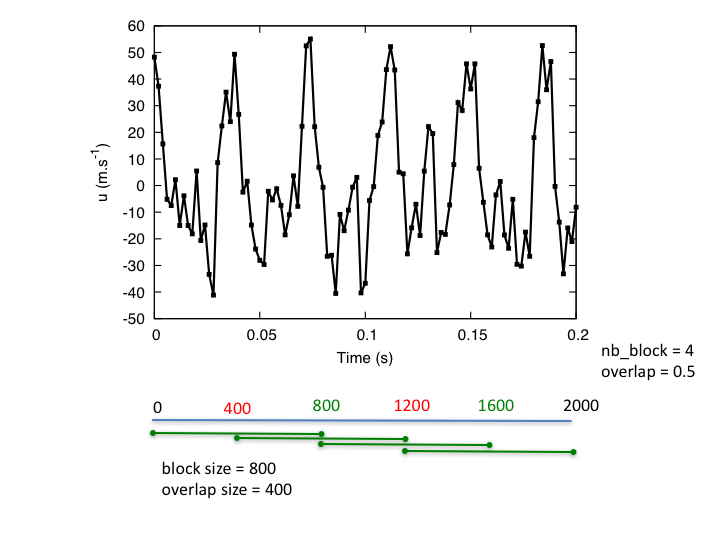
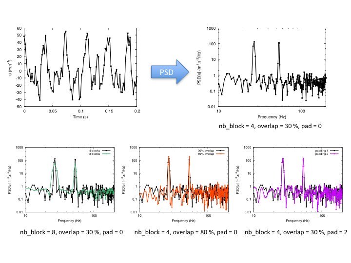
Computes the Power Spectral Density (PSD) of signals using Welch’s average periodogram method. The Welch’s method splits the signal into different overlapping blocks. If needed, a window function might be applied to these blocks, in order to give more weight to the data at the center of the segments. We, then, compute the individual periodogram for each segment by calculating the squared magnitude of the discrete Fourier transform. Finally, the PSD is the average of the individual periodograms.
Note
Dependency on matplotlib.mlab
Parameters
- base:
Base The input base that contains many zones (independent to each others, typically many probes).
- base:
- resize_time_factor: float, default= 1.0
Factor to re-dimensionalize the time variable (time used will be time_var * resize_time_factor). This is useful when you only have the iteration variables and when the time-step used is constant.
- variables: list(str)
The variables that serve as a basis for the PSD. The first variable must be the variable representing time.
- time_t0: float, default= None
Time from which the analysis will start.
- time_tf: float, default= None
Time at which the analysis will end.
- nb_block: int or float, default= 1
Number of Welch’s blocks.
- pad: int or float, default= 1
Padding of the signal with zeros. pad =1 means that there is no padding. Otherwise, if the length of the signal is Ls, then the length of the padded signal will be Ls*pad.
- overlap: int or float, default= 0.33
The percent of the length of the signal to be overlapped.
- window: str or function, default= ‘hanning’
The window function to be applied to each segment. The possible values are: ‘hanning’, ‘none’, ‘blackman’, ‘hamming’, ‘bartlett’.
If none of the above suits you, you can also set your own custom window function. The window function must be a function that accepts a numpy array representing the signal and it returns a single numpy array representing the signal multiplied by the window.
Example : The following code defines a triangular window using the function
triangin thescipy.signallibraryimport scipy.signal def my_triangular_window(signal): return signal * scipy.signal.triang(len(signal)) tt = antares.Treatment('psd') tt['window'] = my_triangular_window
- scale_by_freq: bool, default= True
Whether the resulting density values should be scaled by the scaling frequency, which gives density in units of 1/Hz. This allows for integration over the returned frequency values.
Preconditions
Each zone contains one instant object. Each instant contains at least one 1-D array that represents a time signal.
To change the ordering of variables, you may use base slicing.
Postconditions
The output base contains as many zones as the input base. Each instant contains the following 1-D arrays:
The frequencies (variable named ‘frequency’).
The PSD values for each one of the variables.
Main functions
- class antares.treatment.TreatmentPsd.TreatmentPsd
- execute()
Compute the Power Spectral Density.
- Returns:
a base that contains many zones. Each zone contains one instant. Each instant contains two 1-D arrays:
The values for the power spectrum (real valued)
The frequencies corresponding to the elements in the power spectrum (real valued) (variable ‘frequency’)
- Return type:
Example: impact of options on results
Example
"""
This example illustrates the Power Spectral Density
treatment of Antares. The signal is analyzed on a time window
corresponding to [0.0294, 0.0318].

WARNING, in this case, the file read contains only two
variables, iteration and convflux_ro, the treatment use
the first one as time variable and the second as psd variable.
In case of multiple variables, the first one must be the time variable
and the second one the psd variable. To do so, use base slicing.
"""
import os
import antares

# ------------------
# Reading the files
# ------------------
reader = antares.Reader('column')
reader['filename'] = os.path.join('..', 'data', '1D', 'massflow.dat')
base = reader.read()

# ----
# PSD
# ----
treatment = antares.Treatment('psd')
treatment['base'] = base
treatment['resize_time_factor'] = 3.0E-7
treatment['time_t0'] = 0.0294
treatment['time_tf'] = 0.0318
treatment['variables'] = ['iteration', 'convflux_ro']
result = treatment.execute()

# -------------------
# Plot the result
# -------------------
plot = antares.Treatment('plot')
plot['base'] = result
plot.execute()

# prompt the user
input('press enter to quit')