
Azimuthal decomposition
Error
This treatment is provided by an external module and is not part of the core system. If you’re interested in accessing or utilizing this feature, please contact us for further details and support.
Description
This treatment performs an azimuthal mode decomposition on axial plane.
If \(W(x, r, \theta, t)\) represents the azimuthal evolution at point (x, r) and instant t of the variable of interest, then the mode \(\widehat{W}_m(x,r,t)\) can be computed by the formulas below. If \(\Theta\) is the azimuthal extent (not necessarily \(2\pi\)) of the data then the mode \(m\) corresponds to the frequency \(\frac{m}{\Theta}\). \(N_{\theta}\) (i.e. nb_theta) is the total number of points of the uniform azimuthal discretization and \(\theta_k = \frac{k}{N_{\theta}}\Theta\). The convention that is used depends on the type of the input data (real or complex).
For real input data, \(\widehat{W}_m(x,r,t)\) is defined for positive integers only by:
\(\widehat{W}_0(x,r,t) = \frac{1}{N_{\theta}} \sum_{k=0}^{N_{\theta}} W(x,r,\theta_k,t)\)
\(\widehat{W}_m(x,r,t) = \frac{2}{N_{\theta}} \sum_{k=0}^{N_{\theta}} W(x,r,\theta_k,t) e^{(-i m \theta_k)}\) for \(m >= 1\)
For complex input data, \(W = \operatorname{\mathbb{R}e}\{W\} + i*\operatorname{\mathbb{I}m}\{W\} = \|W\|e^{i \operatorname{arg}(W)}\), \(\widehat{W}_m(x,r,t)\) is defined for both positive and negative integers by:
\(\widehat{W}_m(x,r,t) = \frac{1}{N_{\theta}} \sum_{k=0}^{N_{\theta}} W(x,r,\theta_k,t) e^{(-i m \theta_k)}\)
 ==>
==> 
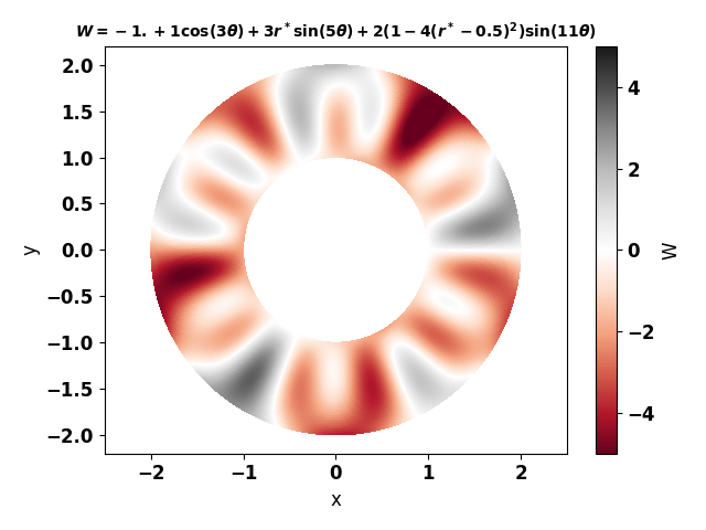
On the left: initial field of \(W\).
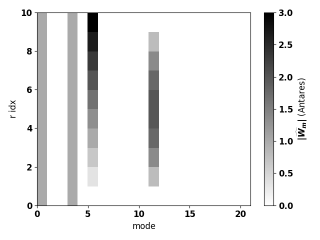
On the right: azimuthal modes \(\|\widehat{W}_m\|\) as a function of the mode and the radial index (see example below).
Construction
import antares
myt = antares.Treatment('AzimModes')
Parameters
- base:
Base The base on which the azimuthal modes will be computed. It can contain several zones and several instants. If dtype_in is ‘re’, then the different instants of the base should correspond to different time iterations. If dtype_in is in [‘mod/phi’, ‘im/re’], then the instants of the base should contain the different time harmonics: ‘Hxx_mod’ and ‘Hxx_phi’ for ‘mod/phi’ or ‘Hxx_re’ and ‘Hxx_im’ for ‘im/re’ (with xx the number of the harmonic), also an instant ‘mean’ containing real data can exist. Decomposition is performed on all variables except coordinates.
- base:
- dtype_in: str, default= ‘im/re’
The decomposition type of the input data: ‘re’ for real data, ‘mod/phi’ for modulus/phase decomposition or ‘im/re’ for imaginery/real part decomposition. If given, the phase must be expressed in degrees.
- dtype_out: str, default= ‘im/re’
The decomposition type of the output data: ‘mod/phi’ for modulus/phase decomposition or ‘im/re’ for imaginery/real part decomposition. The phase is expressed in degrees.
- ring: boolean, default= False
Perform the azimuthal decomposition on the specific case of a microphone azimuthal ring array. Warning: the distributed microphones is supposed to be regularly distributed in azimuthal and radial direction on the ring array.
- coordinates: list(str), default=
antares.Base.coordinate_names The cylindrical coordinates. The angle coordinate must be expressed in radian.
- coordinates: list(str), default=
- x_values: int or list(int) or None, default= None
The axial positions of the planes on which the azimuthal modes are computed. If None, it is assumed that the base is already a plane.
- r_threshold: tuple or None, default= None
Perform the azimuthal decomposition in the defined range of radial values. Useful for multiple coaxial cylinders. The keyword accepts a list of the following structure: [r_var, [(r_min, r_max)]], where r_var is the name of the radius variable. Either r_min or r_max can be None if not limit shall be imposed.
- nb_r: int, default= 20
The number of points in the radial direction of the output base.
- m_max: int, default= 50
The maximum azimuthal mode order to compute. If dtype_in is ‘re’, then ‘m_max’ + 1 modes are computed (from mode 0 to mode ‘m_max’). If dtype_in in [‘mod/phi’, ‘im/re’], then 2 * ‘m_max’ + 1 modes are computed (from mode -‘m_max’ to mode ‘m_max’).
- nb_theta: int, default= 400
The uniform azimuthal line is reconstructed via an interpolation. n_theta is the number of points for this interpolation.
Preconditions
All the zones must have the same instant.
if dtype_in = ‘im/re’ or ‘mod/phi’, instants must be named <harm>_im and <harm>_re or <harm>_mod and <harm>_phi where <harm> is the harmonic. If given, the phase must be expressed in degrees.
Variables must be at nodes, if not the method cell_to_node() is executed.
The input base must be continuous after axial cut but the azimuthal extent can be less than \(2\pi\).
Mesh is not moving.
Postconditions
If dtype_in = ‘mod/phi’, the phase is expressed in degrees.
The result base contain one zone and as much instant than in the input base with suffixes ‘_im’ and ‘_re’ or ‘_mod’ and ‘_phi’. Each variable is a numpy array with dimensions (nb_x, nb_r, m_max + 1) if dtype_in = ‘re’ and with dimensions (nb_x, nb_r, 2 * m_max + 1) else (nb_x is the number of x values).
The azimuthal coordinate is replaced by the azimuthal mode order ‘m’.
Example
The following example shows azimuthal decomposition.
import antares
myt = antares.Treatment('AzimModes')
myt['base'] = base
myt['dtype_in'] = 're'
myt['dtype_out'] = 'mod/phi'
myt['coordinates'] = ['x', 'r', 'theta']
myt['x_values'] = 0.
myt['nb_r'] = 20
myt['r_threshold'] = ['radius', [(None, 0.034948)]]
myt['m_max'] = 50
myt['nb_theta'] = 400
base_modes = myt.execute()
Warning
The frame of reference must be the cylindrical coordinate system. No checking is made on this point.
Main functions
- class antares.plugins.acoustics.treatment.TreatmentAzimModes.TreatmentAzimModes
- execute()
Execute the treatment.
- Returns:
A base that contains one zone. This zone contains several instants. If ‘dtype_in’ is ‘re’, then there are twice as much instants as in the input base (two instants per original instant in order to store seperately modulus and phase or imaginery and real parts). If ‘dtype_in’ is in [‘mod/phi’, ‘im/re’], then there are as many instants in the output base as in the input base. The instant names are suffixed by ‘_mod’ and ‘_phi’ if ‘dtype_out’ is ‘mod/phi’ or by ‘_re’ and ‘_im’ if ‘dtype_out’ is ‘im/re’. Each instant contains the azimuthal modes of the input base variables at different axial and radial positions. The azimuthal coordinate is replaced by the azimuthal mode order ‘m’.
- Return type:
Example
"""
This example shows how to use the azimuthal decomposition treatment.
"""

import antares
import numpy as np
import matplotlib.pyplot as plt

# Define test case
################################################################################
# Geometry
x0 = 0.
rmin, rmax, Nr = 1., 2., 50
tmin, tmax, Nt = 0., 2.*np.pi, 1000
x, r, t = np.linspace(x0, x0, 1), np.linspace(rmin, rmax, Nr), np.linspace(tmin, tmax, Nt)
X, R, T = np.meshgrid(x, r, t)

# Field
r_ = (R - rmin) / (rmax - rmin)
W = -1. +  1.*np.cos(3*T) + 3.*r_*np.sin(5*T) + 2*(1 - 4*(r_ - 0.5)**2)*np.sin(11*T)

# Create antares Base
base = antares.Base()
base['0'] = antares.Zone()
base['0']['0'] = antares.Instant()
base['0']['0']['X'] = X
base['0']['0']['R'] = R
base['0']['0']['T'] = T
base['0']['0']['Y'] = R*np.cos(T)
base['0']['0']['Z'] = R*np.sin(T)
base['0']['0']['W'] = W

# Azimutal decomposition
################################################################################
myt = antares.Treatment('AzimModes')
myt['base'] = base[:,:,('X', 'R', 'T', 'W')]
myt['dtype_in'] = 're'
myt['dtype_out'] = 'mod/phi'
myt['coordinates'] = ['X', 'R', 'T']
myt['x_values'] = None
myt['nb_r'] = 10
myt['m_max'] = 20
myt['nb_theta'] = 800
base_modes = myt.execute()

# Plot data
################################################################################
# font properties
font = {'family':'sans-serif', 'sans-serif':'Helvetica', 'weight':'semibold', 'size':12}

# Plot initial field
t = antares.Treatment('tetrahedralize')
t['base'] = base
base = t.execute()

plt.figure()
plt.rc('font', **font)
plt.tripcolor(base[0][0]['Y'], \
              base[0][0]['Z'], \
              base[0][0].connectivity['tri'], \
              base[0][0]['W'], \
              vmin=-5, vmax=5)
plt.gca().axis('equal')
cbar = plt.colorbar()
cbar.set_label('W')
plt.set_cmap('RdGy')
plt.xlabel('y')
plt.ylabel('z')
plt.title('$W = -1. + 1\\cos(3\\theta) + 3r^*\\sin(5\\theta) + 2(1-4(r^*-0.5)^2)\\sin(11\\theta)$', \
    fontsize=10)
plt.tight_layout()

# Modes computed by antares
mod, phi = base_modes[0]['0_mod'], base_modes[0]['0_phi']

def plot_modes(modes, title='', vmin=0, vmax=1):
    plt.figure()
    plt.rc('font', **font)
    plt.pcolor(modes, vmin=vmin, vmax=vmax)
    cbar = plt.colorbar()
    cbar.set_label(title)
    plt.set_cmap('binary')
    plt.xlabel('mode')
    plt.ylabel('r idx')
    plt.tight_layout()

# Plot modes computed by Antares
plot_modes(modes=mod['W'][0,:,:], title='$\|\\widehat{W}_m\|$ (Antares)', \
    vmin=0, vmax=3)

# Compute analytical solution
mod_th = np.zeros(shape=mod['W'][0,:,:].shape)
mod_th[:,0] = 1.
mod_th[:,3] = 1.
mod_th[:,5] = 3*(mod['R'][0,:,5] - rmin) / (rmax - rmin)
mod_th[:,11] = 2*(1 - 4*((mod['R'][0,:,11] - rmin) / (rmax - rmin) - 0.5)**2)

# Plot analytical solution
plot_modes(modes=mod_th, title='$\|\\widehat{W}_m\|$ (theory)', \
    vmin=0, vmax=3)

# Compute relative error with analytical solution
rel_err = np.abs(mod_th - mod['W'][0,:,:]) / np.max(mod_th) * 100
print('Max relative error between theory and Antares is {:} %.'.format(np.amax(rel_err)))

# Plot relative error with analytical solution
plot_modes(modes=rel_err, title='Relative error with analytical solution [%]', \
    vmin=0, vmax=0.2)

plt.show()