Spectrogram

Description

Computes the Spectrogram of 1D signals.

The spectrogram of signal is computed by dividing the signal into \(N_b\) overlapping blocks of the same length and performing the Fourier transform on each block. This allows us to study the changes of the spectra as a function of time.

Note

Dependency on matplotlib.mlab

Parameters

• base: Base

  The input base. The base can contain many zones, typically, many probes. Each zone must contain the variable(s) on which to compute the spectrogram and the time vector.

• resize_time_factor: float, default= 1.0

  Factor to re-dimensionalize the time variable (time used will be time_var * resize_time_factor). This is useful when you only have the iteration variables and when the time-step used is constant.

• variables: list(str)

  The variables that serve as a basis for the spectrogram. The first variable must be the variable representing time.

• time_t0: float, default= None

  Time from which the analysis will start. If None, the analysis will start from the beginning of the time array.

• time_tf: float, default= None

  Time at which the analysis will end. If :python`None`, the analysis will go until the end of the time array.

• nb_block: int or float, default= 1

  Number of blocks

• pad: int or float, default= 1

  Padding of the signal with zeros. pad =1 means that there is no padding. Otherwise, if the length of the signal is Ls, then the length of the padded signal will be Ls*pad.

• overlap: int or float, default= 0.33

  The percent of the length of the signal to be overlapped.

• window: str or function, default= ‘hanning’

  The window function to be applied to each segment. The possible values are: ‘hanning’, ‘none’, ‘blackman’, ‘hamming’, ‘bartlett’.

  If none of the above suits you, you can also set your own custom window function. The window function must be a function that accepts a numpy array representing the signal and it returns a single numpy array representing the windowed signal.

  • Example : The following code defines a triangular window using the function triang in the scipy.signal library

    import scipy.signal
    
    def my_triangular_window(signal):
        return signal * scipy.signal.triang(len(signal))
    
    tt = antares.Treatment('specgram')
    tt['window'] = my_triangular_window
    

• scale_by_freq: bool or None, default= None

  If the computed spectrogram should be scaled by the sampling frequency. If True the unit of the results will be \(\propto \text{Hz}^{-1}\).

• t_and_f_in_attrs: bool, defaut= True

  If True, the time and frequency vectors will be saved as 1D vectors in the attributes of the instant. If False, they will be saved as 2D matrices resulting from the numpy.meshgrid(time, freq).

• mode: str, default= ‘psd’

  What sort of spectrum to use:

  • 'psd' returns the power spectral density

  • 'complex' returns the complex-valued frequency spectrum

  • 'magnitude' returns the magnitude spectrum

  • 'angle' returns the phase spectrum without unwrapping

  • 'phase' returns the phase spectrum with unwrapping

Preconditions

Each instant must contain all the variables listed in variables.

Postconditions

The output base contains as many zones as the input base. Each zone contains the same number of instant found in the zone of the input base. Each instant contains the variables on which the spectrogram was calculated as a matrix of dimensions \((N_b \times N_f)\), where \(N_b\) is the number of blocks and \(N_f\) is the number of frequencies that can be captured by the Discrete Fourier Transform.

If t_and_f_in_attrs = True the attributes of the instant contain the 'time' and 'frequency’ variables as 1D vectors of length \(N_b\) and \(N_f\). If t_and_f_in_attrs = False, the 'time' and 'frequency’ are stored as 2D matrices of dimensions \((N_b \times N_f)\).

Main functions

class antares.treatment.TreatmentSpecgram.TreatmentSpecgram

execute()

Compute the Power Spectral Density.

Returns:

A base with the same number of zone and instants as the input base and the spectrogram of the variables. Time and frequency can be found either in the attributes of the instant or on the instant’s variables depending on the value of t_and_f_in_attrs.

Return type:

Base

Example

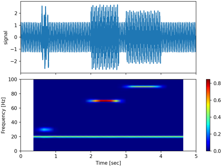
The following example computes the spectrogram of the following 1D signal between \(0 \leq t \leq 5\) with a sampling rate of 10kHz :

\[\begin{split}f\left(t\right) = \sin \left(40 \pi t \right) + \left\{ \begin{array}{lr} 1.5\sin \left(60 \pi t \right) & \text{for } 0.6 \leq t \leq 0.8 \\ 1.5\sin \left(140 \pi t \right) & \text{for } 2.0 \leq t \leq 2.8\\ \sin \left(180 \pi t \right) & \text{for } 3.0 \leq t \leq 4\\ 0 & \text{otherwise} \\ \end{array} \right.\end{split}\]

A random uniform noise of amplitude 0.25 is also added to the signal.

The spectrogram is computed using 30 blocks with an overlap of 80% and no zero-padding. The Hanning window function is used.

import os
import matplotlib.pyplot as plt
import numpy as np

from antares.api import Base
from antares.treatment import Treatment

np.random.seed(19680801)
output_folder = os.path.join(os.getcwd(), 'OUTPUT', 'SPECGRAM')
os.makedirs(output_folder, exist_ok=True)


## Create signal
## =============

dt = 0.0001
time = np.arange(0.0, 5.0, dt)
s1 = 1 * np.sin(2 * np.pi * 20 * time)
s2 = 1.5 * np.sin(2 * np.pi * 30 * time)
s3 = 1.5 * np.sin(2 * np.pi * 70 * time)
s4 = 1.0 * np.sin(2 * np.pi * 90 * time)

# create a transient "chirp"
s2[time < .6] = s2[0.8 <= time] = 0
s3[time < 2.0] = s3[2.8 <= time] = 0
s4[time < 3.0] = s4[4.0 <= time] = 0

# add some noise into the mix
noise = 0.25 * np.random.uniform(-1, 1, size=len(time))

# The signal
signal = s1 + s2 + s3 + s4 + noise

base = Base()
base.init()
base[0][0]['time'] = time
base[0][0]['signal'] = signal

## Spectrogram treatment
## =====================

treatment = Treatment('specgram')
treatment['base'] = base
treatment['variables'] = ['time', 'signal']
treatment['nb_block'] = 30
treatment['pad'] = 1
treatment['overlap'] = 0.8
treatment['t_and_f_in_attrs'] = True
treatment['window'] = 'hanning'
result = treatment.execute()

t = result[0][0].attrs['time']
f = result[0][0].attrs['frequency']
Pxx = result[0][0]['signal']

## Plot spectrogram
## ===============
jet_colormap = plt.cm.get_cmap("jet")

fig, ax = plt.subplots(nrows=2, sharex=True, constrained_layout=True)
_ = ax[0].plot(time, signal)
p = ax[1].pcolormesh(t, f, Pxx, cmap=jet_colormap, shading='gouraud')

plt.xlabel('Time [sec]')
ax[0].set_ylabel('signal')
ax[1].set_ylabel('Frequency [Hz]')

ax[1].set_ylim([0, 100])
ax[1].set_xlim([0, 5])

fig.colorbar(p, ax=ax[1], orientation='vertical')

plt.savefig(os.path.join(output_folder, 'specgram_output.png'), dpi=150)