
Dynamic Mode Decomposition
Description
This processing computes a Dynamic Mode Decomposition (DMD) on 2D/3D field.
The DMD allows to characterize the evolution of a complex non-linear system by the evolution of a linear system of reduced dimension.
For the vector quantity of interest \(v(x_n,t) \in \mathbb{R}^n\) (for example the velocity field of a mesh), where \(t\) is the temporal variable and \(x_n\) the spatial variable. The DMD provides a decomposition of this quantity in modes, each having a complex angular frequency \(\omega_i\):
\(v(x_n,t) \simeq \sum_{i=1}^m c_i \Phi_i(x_n) e^{j \omega_i t}\)
or in discrete form:
\(v_k \simeq \sum_{i=1}^m \lambda_i^k c_i \Phi_i(x_n), \; \mbox{with }\lambda_i^k = e^{j \omega_i \Delta t}\)
with \(\Phi_i\) are the DMD modes.
Using the DMD, the frequencies \(\omega_i\) are obtained with a least-square method.
Compared to a FFT, the DMD has thus the following advantages:
Less spectral leaking
Works even with very short signals (one or two periods of a signal can be enough)
Takes advantage of the large amount of spatial information
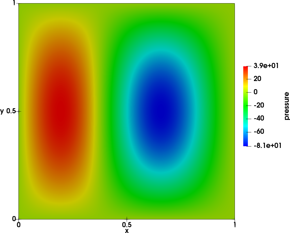
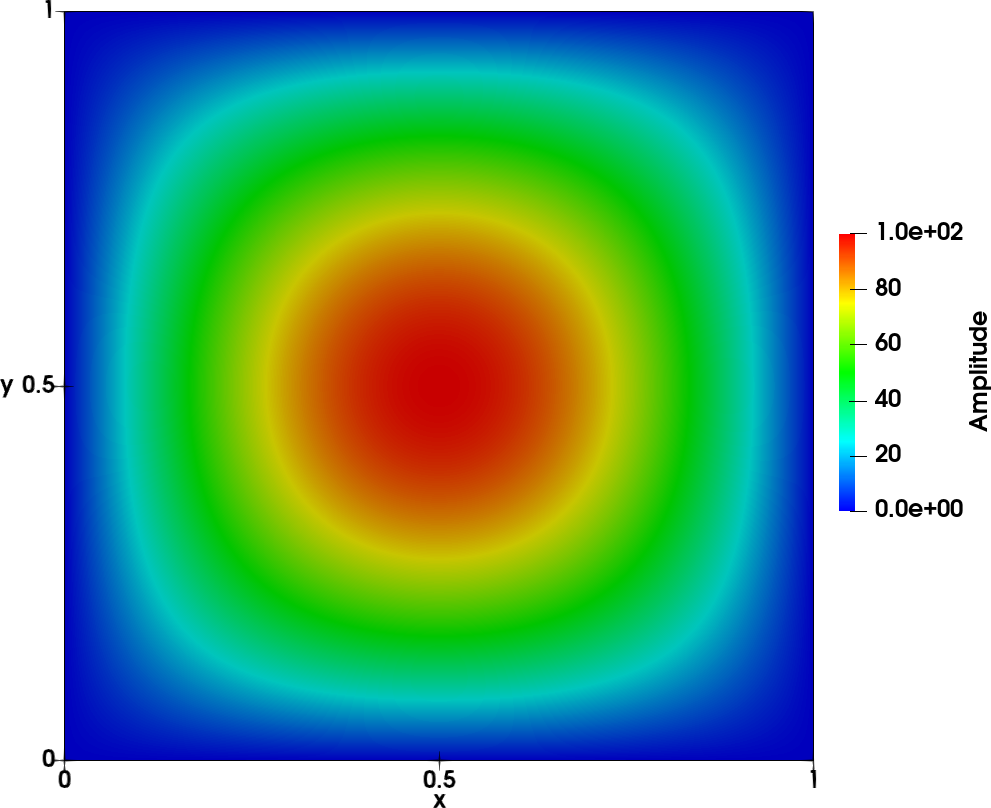
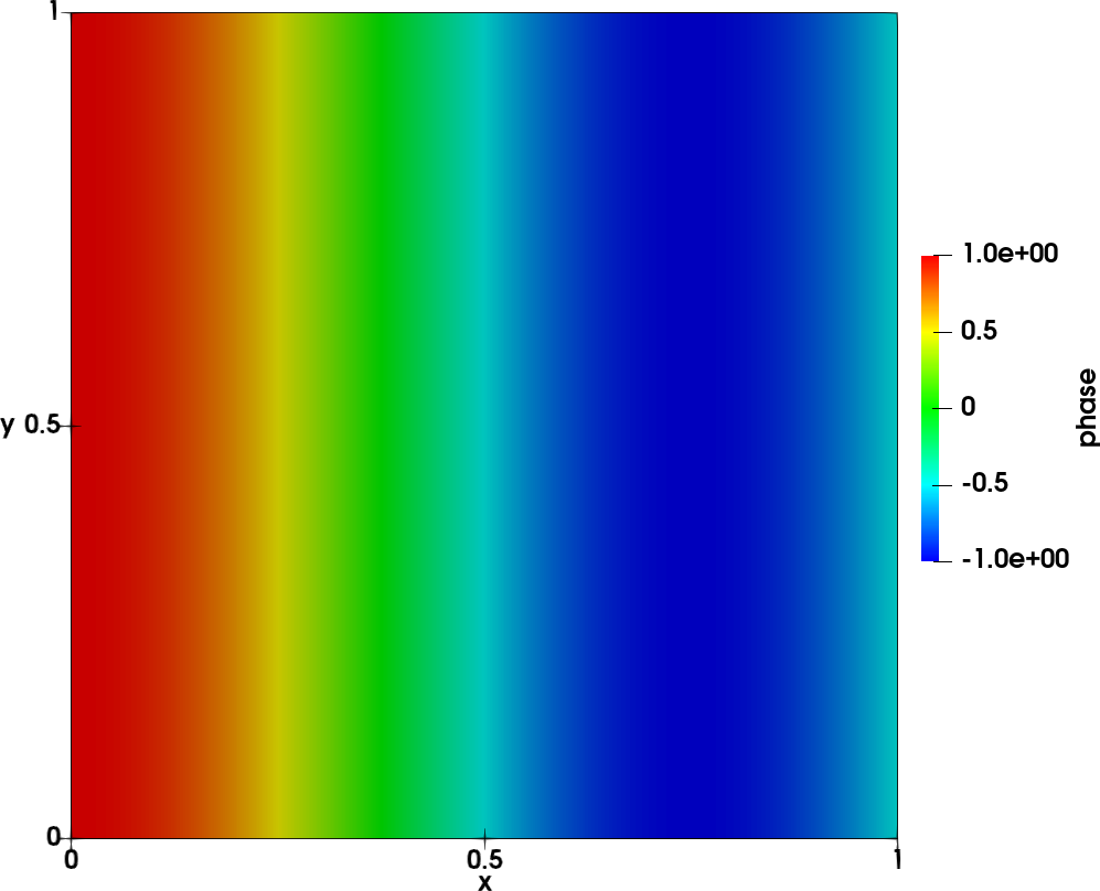
To illustrate the tool, the following reference case is chosen: a wave on a square 2D mesh of size \(100 \times 100\) from \((x,y) = (0,0)\) to \((x,y) = (1,1)\). The unsteady field
\(p(x,y,t) = A sin(n_x \pi x) sin(n_y \pi y) cos(\omega t + \Phi(x))\)
is shown in the left figure below. The amplitude is shown in the middle figure and the phase on the right figure.
- The following parameters are used:
\(A=100\)
\(n_x = n_y = 1\)
\(f = 215 Hz\)
\(\Phi(x) = 4/3 \pi x\)
A database of \(N=100\) snapshots is constructed using a time step \(\Delta t = 2 \times 10^{-4} s\), leading to a Nyquist frequency \(f_e = 1/2\Delta t = 2500 Hz\) and a resolution \(\Delta f = 1/N\Delta=50 Hz\).
Using the DMD algorithm, the spectrum and amplifications obtained are shown in the figures below:
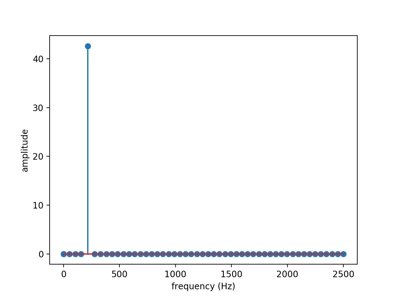
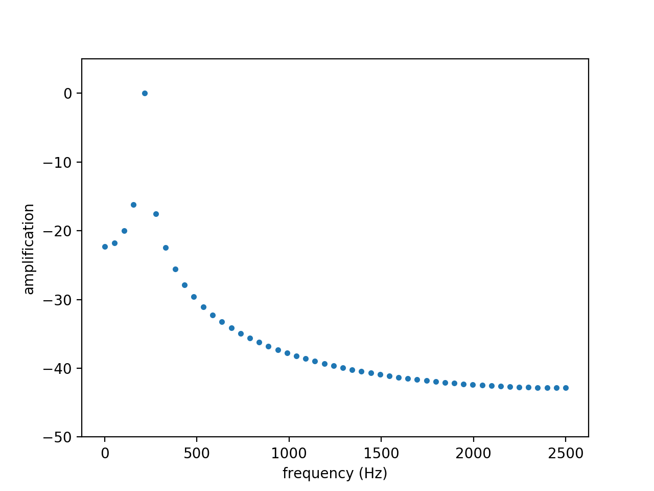
The exact value of 215 Hz expected from the frequency peak is present on the amplitude spectrum. The amplification is very close to zero, which is expected since the wave is neither amplified nor attenuated.
Construction
import antares
myt = antares.Treatment('dmd')
Parameters
- base:
Base The input base that contains one zone which contains one instant. The instant contains at least two 2-D arrays that represent the cell volumes and a scalar value.
- base:
- time_step: float
The time step between two instants \(\Delta t\).
- noiselevel: float, default= 1e-9
The noise level should be increased when ill-conditioned and non-physical modes appear.
- type: str, default= ‘mod/phi’
The decomposition type of the DMD:
mod/phi for modulus/phase decomposition or
im/re for imaginery/real part decomposition.
- variables: list(str)
The variable names. The variable representing the volume of each cell must be the first variable in the list of variables. The other variables are the DMD variables.
- memory_mode: bool, default= False
If True, the initial base is deleted on the fly to limit memory usage.
- list_freq: list(float), default= []
Frequency peaks to detect in Hertz. If no specific frequency is given, the DMD will be achieved on all modes (costly).
- delta_freq: float, default= 0
The frequential resolution of the base, ie \(\Delta f = 1/T\), with \(T\) the total time of the database (\(T = \mbox{number of instants} \times \Delta t\))
Preconditions
The input base must be an unstructured mesh.
The variable representing the volume of each cell must be the first variable in the list of variables. The other variables are the DMD variables.
Moreover, the frequential resolution of the base must be \(\Delta f = 1/T\) in Hertz, with \(T\) the total time of the database (\(T = \mbox{number of instants} \times \Delta t\)).
Postconditions
The treatment returns one output base containing:
a zone named ‘spectrum’ with an instant named ‘spectrum’ with three variables ‘frequency’, ‘amplification’, and ‘p_modulus’ (magnitude)
a zone named ‘modes’. Each DMD variable modes will be stored in different instants. Each instant contains two variables depending on the type of DMD (e.g. ‘p_mod’ and ‘p_phi’)
The output zone ‘modes’ contains some keys ‘peak_modes_<variable name>’ in its
Zone.attrs. These peak modes are the name of instants in the zone.
Each instant in the output zone ‘modes’ contains two keys ‘frequency’ and
‘amplification’ in its Instant.attrs.
References
P. J. Schmid: Dynamic mode decomposition of numerical and experimental data. J. Fluid Mech., vol. 656, no. July 2010, pp. 5–28, 2010.
Example
import antares
treatment = antares.Treatment('dmd')
treatment['time_step'] = 0.1
treatment['variables'] = ['volumes', 'pressure', 'vx']
treatment['noiselevel'] = 1e-4
treatment['base'] = base
treatment['list_freq'] = [300.0, 600.0]
treatment['delta_freq'] = 50.0
treatment['type'] = 'im/re'
result = treatment.execute()
Main functions
Example
"""
This example illustrates the Dynamic Mode Decomposition.
It is a stand alone example : the Base used for the DMD
is not read in a file, it is created in the example
"""
import os
import numpy as np
from antares import Base, Instant, Treatment, Writer, Zone


def myfunc(x, y, t, A, w, Phi):
    return A * np.sin(np.pi*x)*np.sin(np.pi*y)*np.cos(w*t+Phi*x)


if not os.path.isdir('OUTPUT'):
    os.makedirs('OUTPUT')

# ----------------------
# Create the input base
# ----------------------

# Initial parameters
time_step = 2e-4
nb_snapshot = 50
T = nb_snapshot*time_step
A1 = 100.0
A2 = 10.0
f1 = 215.0
f2 = 120.0
w1 = f1*2.0*np.pi
w2 = f2*2.0*np.pi
Phi = 4.0/3.0*np.pi

# Create a 2D mesh
n = 50
mgrid = np.mgrid[0:n, 0:n]
xt = (mgrid[0]/(n-1.))
yt = (mgrid[1]/(n-1.))

# Initialise the base
base = Base()
base['zone_0'] = Zone()
base[0].shared['x'] = xt
base[0].shared['y'] = yt
base.unstructure()

# Define the cell volume
ncell = base[0].shared['x'].shape[0]
volume = np.ones((ncell))
base[0].shared['cell_volume'] = volume

# Extract coordinates and define time
x = base[0].shared['x']
y = base[0].shared['y']
time = np.linspace(0.0, T, nb_snapshot)

# Generate temporal database
for snapshot_idx in range(nb_snapshot):
    instant_name = 'snapshot_%s' % snapshot_idx
    base[0][instant_name] = Instant()
    base[0][instant_name]['pressure'] = myfunc(x, y, time[snapshot_idx], A1, w1, Phi)
    base[0][instant_name]['vx'] = myfunc(x, y, time[snapshot_idx], A2, w2, Phi)

# --------------
# DMD treatment
# --------------
treatment = Treatment('Dmd')
treatment['time_step'] = time_step
treatment['variables'] = ['cell_volume', 'pressure', 'vx']
treatment['noiselevel'] = 1e-9
treatment['base'] = base
treatment['list_freq'] = [f1, f2]
treatment['delta_freq'] = 50.0
treatment['type'] = 'im/re'
result = treatment.execute()

# -------------------
# Writing the result
# -------------------

# Write the spectrum (frequency, magnification and magnitude)
writer = Writer('column')
writer['filename'] = os.path.join('OUTPUT', 'ex_dmd_spectrum.dat')
writer['base'] = result[('spectrum', )]
writer.dump()

# Pick and write modes: here we retreive the peak modes of pressure for each variables
peak_modes = result['modes'].attrs['peak_modes_pressure']
newbase = result[('modes', ), peak_modes]
newbase[0].shared.connectivity = base[0][0].connectivity
newbase[0].shared['x'] = base[0][0]['x']
newbase[0].shared['y'] = base[0][0]['y']
writer = Writer('bin_tp')
writer['filename'] = os.path.join('OUTPUT', 'ex_dmd_pressure_peak_mode_<instant>.plt')
writer['base'] = newbase
writer.dump()

# Pick and write modes: here we retreive the peak modes of velocity for each variables
peak_modes = result['modes'].attrs['peak_modes_vx']
newbase = result[('modes', ), peak_modes]
newbase[0].shared.connectivity = base[0][0].connectivity
newbase[0].shared['x'] = base[0][0]['x']
newbase[0].shared['y'] = base[0][0]['y']
writer = Writer('bin_tp')
writer['filename'] = os.path.join('OUTPUT', 'ex_dmd_vx_peak_mode_<instant>.plt')
writer['base'] = newbase
writer.dump()

# Write the effective frequencies of identified modes
fic = open(os.path.join('OUTPUT', 'ex_dmd_list_modes.dat'), 'w')
for key in result[('modes', ), peak_modes][0].keys():
    fic.write(key)
    fic.write('\t')
    fic.write(str(result[('modes', ), peak_modes][0][key].attrs['frequency']))
    fic.write('\n')