
Averaged Meridional Plane
Description
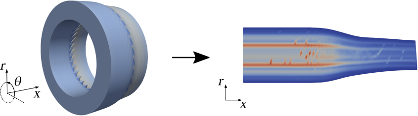
Compute an averaged meridional plane of a turbomachine at steady-state.
The azimuthal averages are performed using a surface thermodynamic average on small surfaces that are normal to the curvilinear abscissa of the machine.
Construction
import antares
myt = antares.Treatment('averagedmeridionalplane')
Parameters
- base:
Base The input base on which the meridional plane is built.
- base:
- cartesian_coordinates:
list(str), default= [‘x’, ‘y’, ‘z’] Ordened names of the cartesian coordinates.
- cartesian_coordinates:
- merid_coordinates:
list(str), default= [‘x’, ‘r’] Names of the meridional plane coordinates: the axis of rotation (axial coordinate) and the distance to this axis (radius).
- merid_coordinates:
- machine_coordinates:
list(str), default= [‘x’, ‘r’, ‘theta’] Names of three coordinates related to the machine: a curvilinear abscissa, a height coordinate and an azimuthal coordinate. It usually depends on the type of machine processed. The curvilinear abscissa is used as the normal to the small averaging surfaces.
- machine_coordinates:
- out_coordinates:
list(str), default= [‘x’, ‘y’, ‘z’] Names of the coordinates in the output Base. The two first are the meridional plane coordinates.
- out_coordinates:
- out_variables:
list(str), default= [] Names of the output averaged variables contained in the output Base.
- out_variables:
- cut_treatment:
Treatment A preconfigured cut treatment, used to perform cuts of the 3D volume within the algorithm.
- cut_treatment:
- thermo_treatment:
Treatment A preconfigured thermodynamic average treatment, used to average the output variables merid_coordinates and out_variables on 2D surfaces.
- thermo_treatment:
- abscissa_nb:
int, default= 50 Number of curvilinear abscissas (first component of machine_coordinates) taken to discretize the meridional plane.
- abscissa_nb:
- abscissa_distrib:
strin [‘uniform’, ‘normal’], default= ‘uniform’ Distribution of the discretization of the curvilinear abscissa.
- abscissa_distrib:
- height_nb:
int, default= 20 Number of heights (second component of machine_coordinates) taken to discretize the meridional plane.
- height_nb:
- height_distrib:
strin [‘uniform’, ‘normal’], default= ‘normal’ Distribution of the discretization of the height coordinate.
- height_distrib:
Preconditions
The input base must fulfill the preconditions of the input thermo_treatment, except the mono-zone requirement. The base is mono-instant (steady-state).
The merid_coordinates and the machine_coordinates must be available in the input base at nodes.
The given cut treatment must have an input called base, an input type which is the geometrical type of cut that can take the ‘plane’ value, an input coordinates, the system of coordinates used, an input normal, the normal vector of the plane cut and an input origin, a point such that the cut plane passes through.
The given thermodynamic average must have an input called base, a 2D surface, an input def_points allowing to define the normal of the surface, and an output dictionnary called ‘0D/AveragedMeridionalPlane’ containing the variables given in merid_coordinates and out_variables.
The abscissa_nb and the height_nb must be greater or equal to 1.
Postconditions
The output is a new mono-zone and mono-instant Base containing the computed meridional plane with coordinates called out_coordinates and variables called out_variables located at nodes.
The input base is unchanged.
Example
import antares
import numpy as np

# code that creates a Base fulfilling the preconditions
# it is a structured approximation of an annulus (r_min = 1.0, r_max = 2.0,
# pitch = pi/2) extruded from x = 0.0 to x = 1.0
# having Cartesian coordinates called 'x', 'y', 'z'
# having machine coordinates called 'x', 'r', 'theta'
base = antares.Base()
base.init()
base[0][0]['x'] = [[[0.0, 0.0], [0.0, 0.0]], [[1.0, 1.0], [1.0, 1.0]]]
base[0][0]['r'] = [[[1.0, 2.0], [1.0, 2.0]], [[1.0, 2.0], [1.0, 2.0]]]
base[0][0]['theta'] = [[[0.0, 0.0], [np.pi/2.0, np.pi/2.0]], [[0.0, 0.0],
                        [np.pi/2.0, np.pi/2.0]]]
base.compute('y = r*cos(theta)')
base.compute('z = r*sin(theta)')
# having conservative variables called rho, rhou, rhov, rhow, rhoE at nodes
base[0][0]['rho'] = [[[1.0, 1.0], [1.0, 1.0]], [[1.2, 1.2], [1.2, 1.2]]]
base[0][0]['rhou'] = [[[1.0, 1.0], [1.0, 1.0]], [[1.0, 1.0], [1.0, 1.0]]]
base[0][0]['rhov'] = [[[0.0, 0.0], [0.0, 0.0]], [[0.0, 0.0], [0.0, 0.0]]]
base[0][0]['rhow'] = [[[0.0, 0.0], [0.0, 0.0]], [[0.0, 0.0], [0.0, 0.0]]]
base[0][0]['rhoE'] = [[[1.0e5, 1.0e5], [1.0e5, 1.0e5]], [[1.0e5, 1.0e5],
                       [1.0e5, 1.0e5]]]
# having gas properties and row properties as attributes (mono-row case)
# the row rotates at 60 rpm
base.attrs['Rgas'] = 250.0
base.attrs['gamma'] = 1.4
base.attrs['omega'] = 2.0*np.pi
base.attrs['pitch'] = np.pi/2.0

# construction and configuration of the cut treatment used by the algo
t_cut = antares.Treatment('cut') # VTK-triangles

# construction and configuration of the thermo average treatment
t_thermo = antares.Treatment('thermo7')
t_thermo['cylindrical_coordinates'] = ['x', 'r', 'theta']
t_thermo['conservative'] = ['rho', 'rhou', 'rhov', 'rhow', 'rhoE']

# computation of the averaged meridional plane
t = antares.Treatment('averagedmeridionalplane')
t['base'] = base
t['cartesian_coordinates'] = ['x', 'y', 'z']
t['merid_coordinates'] = ['x', 'r']
t['machine_coordinates'] = ['x', 'r', 'theta']
t['out_variables'] = ['alpha', 'beta', 'phi', 'Ma', 'Mr', 'Psta', 'Pta',
                      'Ptr', 'Tsta', 'Tta', 'Ttr']
t['cut_treatment'] = t_cut
t['thermo_treatment'] = t_thermo
t['abscissa_nb'] = 2
t['height_nb'] = 3
base_merid = t.execute()

# export the averaged meridional plane
w = antares.Writer('hdf_antares')
w['filename'] = 'my_averaged_meridional_plane'
w['base'] = base_merid
w.dump()