
Bi-Periodic Plane Channel Initialization
Description
Create the mesh and the initial condition (white noise or spanwise vortices) for a plane channel flow.
Construction
import antares
myt = antares.Treatment('initchannel')
Parameters
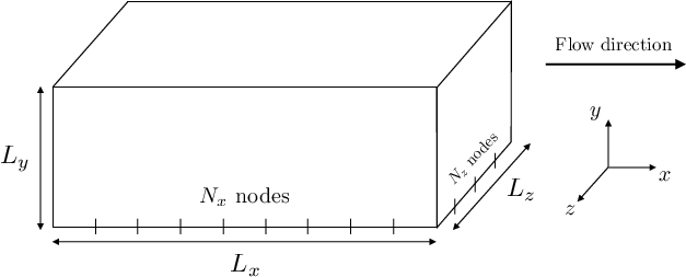
- domain_size: list(int)
Size of the channel in longitudinal (Lx), normal (Ly), and transverse (Lz) directions.
- mesh_node_nb: list(int)
Number of nodes used to create the mesh in the longitudinal (Nx), normal (Ny), and transverse (Nz) directions
- stretching_law: str, default= ‘uniform’
The stretching law used in the wall-normal direction. 4 laws are available: ‘uniform’ (default), ‘geometric’, ‘tanh1’, and ‘tanh2’.
- ratio: float, default= 1.
The expansion ratio (r) of the cells size in the wall-normal direction in case of non-uniform stretching.
- perturbation_amplitude: list(float), default= [0.05, 0.]
White noise amplitude in the longitudinal direction and vortex amplitude. White noise amplitude in the other directions is equal to 2 times this value.
- bulk_values: list(float), default= [0.05, 0.]
Bulk velocity in the longitudinal direction and bulk density.
- t_ref: float,
Temperature of reference.
- cv: float,
Specific heat coefficient at constant volume.
Preconditions
Postconditions
The returned base contains one structured zone with one instant with default names. It contains the mesh at nodes and conservative variables (ro, rou, rov, row, roE) at cell centers. The following attributes are stored in the base: Distance from the wall of the first row nodes y_1 = \(\Delta y_1\), uniform grid spacings \(\Delta x\) and \(\Delta z\), and grid spacing at the channel center \(\Delta y_c\).
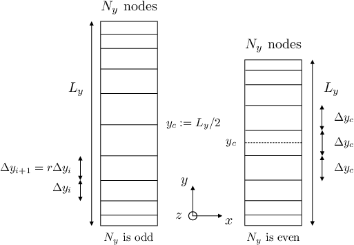
The mesh can be uniform or stretched in the wall-normal direction thanks to the ratio parameter r (1<r<1.05). According to the parity of nodes number Ny in the wall-normal direction, the center of the cell y_c is either on a cell (even case) or on a node (odd case). In the even case, \(\Delta y_1\) is computed such that \(\Delta y_c\) is equal to its neighboring values. So given N_y and r:
the first hyperbolic tangent law is defined by: \(\displaystyle \forall i \leq N_y - 1, y_i = \frac{1}{r} \tanh(\xi_i atanh(r)) + 1\) with \(\xi_i = -1 + 2 \frac{i}{N_y - 1}\) and \(0 < r < 1\).
This law has been used by Moin and Abe
the second hyperbolic tangent law is defined by: \(\displaystyle \forall i \leq N_y - 1, y_i = 1 - \frac{\tanh(r \xi_i)}{\tanh(r)}\) with \(\xi_i = 1 - 2 \frac{i}{N_y - 1}\).
It has been used by Gullbrand.
the geometric stretching is defined by: \(\displaystyle \frac{\Delta y_{i+1}}{\Delta y_i} = r\)
It is advised to choose \(r \in [1;1.05]\). According to the parity of nodes number Ny in the wall-normal direction, the center of the cell y_c is either on a cell (even case) or on a node (odd case). In the even case, \(\Delta y_1\) is computed such that \(\Delta y_c\) is equal to its neighboring values. So given N_y and r:
\(\displaystyle \Delta y_1 = \frac{L_y}{2} \frac{1-r}{1-r^{\frac{N_y-1}{2}}}\) if Ny is odd
\(\displaystyle \Delta y_1 = \frac{L_y}{2}\frac{1-r}{1-r^{N_y/2-1}} \frac{1}{1+\frac{(1-r)r^{N_y/2-2}}{2(1-r^{N_y/2-1})}}\) if Ny is even
Of course, \(\Delta y = L_y / (N_y - 1)\) if r = 1.
The initial condition is based on a power law for the longitudinal velocity \(u(y)= \frac{8}{7} u_b \left( 1 - \lvert{1 - \frac{y}{h}\rvert}\right)^{1/7}\) with \(u_b\) the bulk velocity.
The density \(\rho\) is chosen uniform, and equals to the bulk density \(\rho_b\).
To ease the transition to turbulence, one can add:
a white noise which maximum level in the streamwise direction equal to twice those in the wall-normal and spanwise directions
or/and vortex rings as used by LeBras.
It is not recommended to mix them. A white noise is enough on coarse mesh while vortex rings are well-suited to fine grid. The initial temperature should be chosen to the wall temperature to avoid entropy waves.
Perturbations are added to the power law velocity:
\(u_\text{pert} = \alpha u_b \frac{y-y_0}{b} \exp\left(-\frac{a^2\ln2}{b^2}\right) \left(1+0.5 |\sin(\frac{4\pi z}{L_z})|\right)\)
\(v_\text{pert} = -\alpha u_b \frac{x-x_0}{b} \exp\left(-\frac{a^2\ln2}{b^2}\right) \left(1+0.5 |\sin(\frac{4\pi z}{L_z})|\right)\)
with:
\(x_0\) and \(y_0=0.3 L_y/2\) the coordinates of the center vortex
\(\alpha\) a constant which represents the amplitude and can be set with the perturbation_amplitude parameter (0.6 advised, and 0. by default)
\(a=\sqrt{(x-x_0)^2+(y-y_0)^2}\)
\(b=4\Delta_x\)
Vortex rings are spaced \(20\Delta_x\) in the longitudinal direction.
Refences
P. Moin and J. Kim (1982). “Numerical investigation of turbulent channel flow”. In: Journal of Fluid Mechanics, 118, pp 341-377
H. Abe et al. (2001). “Direct Numerical Simulation of a Fully Developed Turbulent Channel Flow With Respect to the Reynolds Number Dependence”. In: Journal of Fluids Engineering, 123, pp 382-393.
J. Gullbrand (2003). “Grid-independent large-eddy simulation in turbulent channel flow using three-dimensional explicit filtering”. In: Center for Turbulence Research Annual Research Briefs.
S. Le Bras et al. (2015). “Development of compressible large-eddy simulations combining high-order schemes and wall modeling”. In: AIAA Aviation, 21st AIAA/CEAS Aeroacoustics Conference. Dallas, TX.
Main functions
Example
import math
import os

import antares

if not os.path.isdir('OUTPUT'):
    os.makedirs('OUTPUT')

gam = 1.4
mach = 0.2

t = antares.Treatment('initchannel')
t['domain_size'] = [2*math.pi, 2., math.pi]  # [Lx,Ly,Lz]
t['mesh_node_nb'] = [49, 41, 41]  # [Nx,Ny,Nz]
t['ratio'] = 1.0  # stretch ratio in wall-normal direction
t['stretching_law'] = 'uniform'
# Flow init parameter
t['bulk_values'] = [1., 1.]  # bulk velocity and bulk density
t['perturbation_amplitude'] = [0., 0.6]  # [white noise=0.05,vortex rings=0.] by default
t['t_ref'] = 1.0
t['cv'] = 1./(gam*(gam-1)*mach**2)

b = t.execute()

# w = ant.Writer()
# w['filename'] = 'mesh'
# w['file_format'] = 'fmt_tp'
# w['base'] = b[:,:,('x','y','z')]
# w.dump()

w = antares.Writer('fmt_tp')
w['filename'] = os.path.join('OUTPUT', 'ex_flow_init_channel.dat')
w['base'] = b[:, :, (('x', 'cell'), ('y', 'cell'), ('z', 'cell'),
                     'ro', 'rovx', 'rovy', 'rovz', 'roE')]
w.dump()