
Radial decomposition
Error
This treatment is provided by an external module and is not part of the core system. If you’re interested in accessing or utilizing this feature, please contact us for further details and support.
Description
This treatment computes the radial modes (useful for duct acoustics) by a projection of each azimuthal mode over the radial eigenfunctions (combinaison of Bessel functions of first and second kinds).
It must be used after computing the azimuthal modes (with the Azimuthal Mode
Decomposition treatment antares.treatment.TreatmentAzimModes).
If \(\hat{W}_{m}(x,r,t)\) denotes the radial
evolution of the azimuthal mode of order \(m\) (with
\(R_{min} < r < R_{max}\)), then the radial modes
\(\hat{W}_{mj}(x,t)\) (where \(j\) is the radial mode order) are given by
\(\hat{W}_{mj}(x,t) = \frac{2}{R_{max}^{2}-R_{min}^{2}} \int_{R_{min}}^{R_{max}} \hat{W}_{m}(x,r,t) E_{mj}(x,r) r dr\).
The radial eigenfunctions \(E_{mj}(x,r)\) are expressed as
\(E_{mj}(x,r) = A_{mj}(x) J_{m}(K_{mj}(x) r) + B_{mj}(x) Y_{m}(K_{mj}(x) r)\),
where \(J_{m}\) and \(Y_{m}\) are the Bessel functions of order \(m\) of first and second kinds respectively and \(A_{mj}\), \(B_{mj}\) and \(K_{mj}\) are duct coefficients (depending on the minimum and maximum duct radius \(R_{min}\) and \(R_{max}\)).
 ==>
==>  ==>
==> 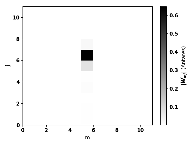
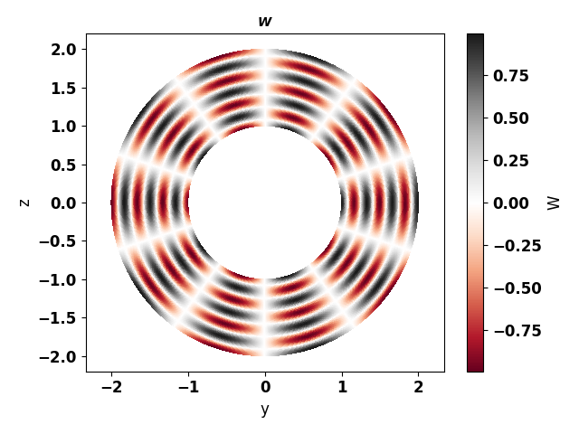
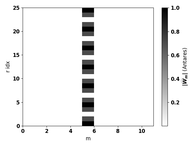
From left to right: initial field \(W\), azimuthal modes \(\|\widehat{W}_m\|\)
computed with antares.treatment.TreatmentAzimModes and
radial modes \(\|\widehat{W}_{mj}\|\)
computed with the radmodes treatment.
Construction
import antares
myt = antares.Treatment('RadModes')
Parameters
- base:
Base The input base on which the radial mode decomposition will be done. It must result from the Azimuthal Mode Decomposition treatment. It should therefore contain one zone with several instants. The instant names should be suffixed by ‘_mod’ and ‘_phi’ if dtype_in is ‘mod/phi’ or by ‘_re’ and ‘_im’ if dtype_in is ‘im/re’. The first three variables of each instant should be the axial coordinate, the radial coordinate and the azimuthal mode order ‘m’ (in this order). The other variables are the ones on which the decomposition will be done.
- base:
- dtype_in: str, default= ‘im/re’
The decomposition type of the input data: ‘mod/phi’ for modulus/phase decomposition or ‘im/re’ for imaginery/real part decomposition. If given, the phase must be expressed in degrees.
- dtype_out: str, default= ‘im/re’
The decomposition type used for the output data: ‘mod/phi’ for modulus/phase decomposition or ‘im/re’ for imaginery/real part decomposition. If given, the phase is expressed in degrees.
- j_max: int, default= 10
The maximum radial mode order to compute (j_max + 1 modes are computed).
Preconditions
The input base has to be constructed by the treatment azimmodes
(antares.treatment.TreatmentAzimModes).
Postconditions
The output base contains one zone and as much instant as in the input base with suffixes ‘_im’ and ‘_re’ or ‘_mod’ and ‘_phi’. Each variable is a numpy array with dimensions (nb_x, j_max + 1, nb_m) where nb_x is the number of x values and nb_m is the number of azimuthal modes of the input base.
The radial coordinate is replaced by the radial mode order ‘j’.
Example
The following example shows radial decomposition.
import antares
myt = antares.Treatment('RadModes')
myt['base'] = base_azimmodes
myt['dtype_in'] = 'mod/phi'
myt['dtype_out'] = 'mod/phi'
myt['j_max'] = 10
base_radmodes = myt.execute()
Warning
The frame of reference must be the cylindrical coordinate system. No checking is made on this point.
Main functions
- class antares.plugins.acoustics.treatment.TreatmentRadModes.TreatmentRadModes
- execute()
Execute the treatment.
- Returns:
A base that contains one zone. This zone contains as many instants as in the input base. The instant names are suffixed by ‘_mod’ and ‘_phi’ if ‘dtype_out’ is ‘mod/phi’ or by ‘_re’ and ‘_im’ if ‘dtype_out’ is ‘im/re’. Each instant contains the radial modes of the input base variables for all provided azimuthal mode orders and axial positions. The radial coordinate is replaced by the radial mode order ‘j’.
- Return type:
Example
"""
This example shows how to use the radial decomposition treatment.
"""

import antares
import numpy as np
import matplotlib.pyplot as plt

# Define test case
################################################################################
# Geometry
x0 = 0.
rmin, rmax, Nr = 1., 2., 100
tmin, tmax, Nt = 0., 2.*np.pi, 1000
x, r, t = np.linspace(x0, x0, 1), np.linspace(rmin, rmax, Nr), np.linspace(tmin, tmax, Nt)
X, R, T = np.meshgrid(x, r, t)

# Field
r_ = R / (rmax - rmin)
W = np.cos(2*np.pi*3*r_)*np.cos(5*T)

# Create antares Base
base = antares.Base()
base['0'] = antares.Zone()
base['0']['0'] = antares.Instant()
base['0']['0']['X'] = X
base['0']['0']['R'] = R
base['0']['0']['T'] = T
base['0']['0']['Y'] = R*np.cos(T)
base['0']['0']['Z'] = R*np.sin(T)
base['0']['0']['W'] = W

# Azimutal decomposition
################################################################################
myt = antares.Treatment('AzimModes')
myt['base'] = base[:,:,('X', 'R', 'T', 'W')]
myt['dtype_in'] = 're'
myt['dtype_out'] = 'mod/phi'
myt['coordinates'] = ['X', 'R', 'T']
myt['x_values'] = None
myt['nb_r'] = 25
myt['m_max'] = 10
myt['nb_theta'] = 800
base_modes = myt.execute()

# Plot data
################################################################################
# font properties
font = {'family':'sans-serif', 'sans-serif':'Helvetica', 'weight':'semibold', 'size':12}

# Plot initial field
t = antares.Treatment('tetrahedralize')
t['base'] = base
base = t.execute()

plt.figure()
plt.rc('font', **font)
plt.tripcolor(base[0][0]['Y'], \
              base[0][0]['Z'], \
              base[0][0].connectivity['tri'], \
              base[0][0]['W'])
plt.gca().axis('equal')
cbar = plt.colorbar()
cbar.set_label('W')
plt.set_cmap('RdGy')
plt.xlabel('y')
plt.ylabel('z')
plt.title('$W$', \
    fontsize=10)
plt.tight_layout()

# Modes computed by antares
mod, phi = base_modes[0]['0_mod'], base_modes[0]['0_phi']

def plot_modes(modes, title='', xlabel='', ylabel=''):
    plt.figure()
    plt.rc('font', **font)
    plt.pcolor(modes)
    cbar = plt.colorbar()
    cbar.set_label(title)
    plt.set_cmap('binary')
    plt.xlabel(xlabel)
    plt.ylabel(ylabel)
    plt.tight_layout()

# Plot modes computed by Antares
plot_modes(modes=mod['W'][0,:,:], title='$\|\\widehat{W}_m\|$ (Antares)', xlabel='m', ylabel='r idx')

# Radial decomposition
################################################################################
myt = antares.Treatment('RadModes')
myt['base'] = base_modes
myt['dtype_in'] = 'mod/phi'
myt['dtype_out'] = 'mod/phi'
myt['j_max'] = 10
base_radmodes = myt.execute()

# Modes computed by antares
mod, phi = base_radmodes[0]['0_mod'], base_radmodes[0]['0_phi']

# Plot modes computed by Antares
plot_modes(modes=mod['W'][0,:,:], title='$\|\\widehat{W}_{mj}\|$ (Antares)', xlabel='m', ylabel='j')

plt.show()