
Signal Dynamic Mode Decomposition (1-D signals)
Description
This processing computes a Dynamic Mode Decomposition (DMD) of a 1D signal.
The DMD allows to characterize the evolution of a complex non-linear system by the evolution of a linear system of reduced dimension.
For the vector quantity of interest \(v(x_n,t) \in \mathbb{R}^n\) (for example the velocity field at a node of a mesh), where \(t\) is the temporal variable and \(x_n\) the spatial variable. The DMD provides a decomposition of this quantity in modes, each having a complex angular frequency \(\omega_i\):
\(v(x_n,t) \simeq \sum_{i=1}^m c_i \Phi_i(x_n) e^{j \omega_i t}\)
or in discrete form:
\(v_k \simeq \sum_{i=1}^m \lambda_i^k c_i \Phi_i(x_n), \; \mbox{with }\lambda_i^k = e^{j \omega_i \Delta t}\)
with \(\Phi_i\) the DMD modes.
Using the DMD, the frequencies \(\omega_i\) are obtained with a least-square method.
Compared to a FFT, the DMD has thus the following advantages:
Less spectral leaking
Works even with very short signals (one or two periods of a signal can be enough)
Takes advantage of the large amount of spatial information
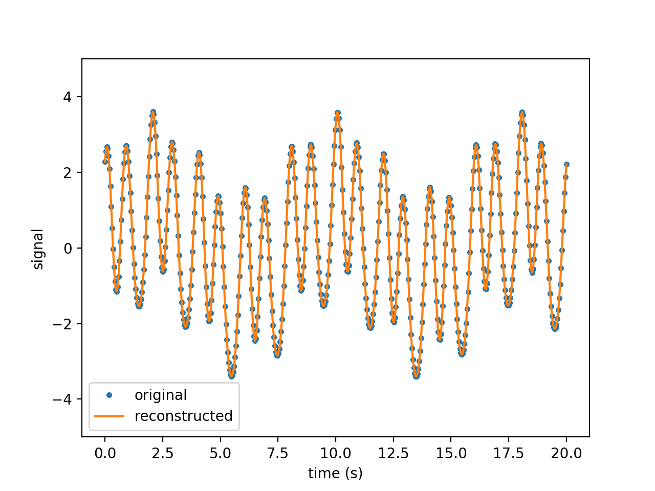
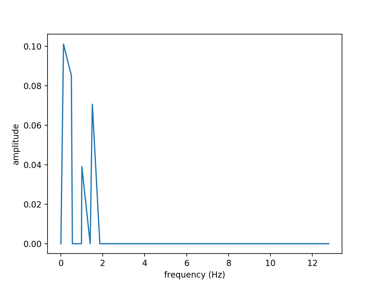
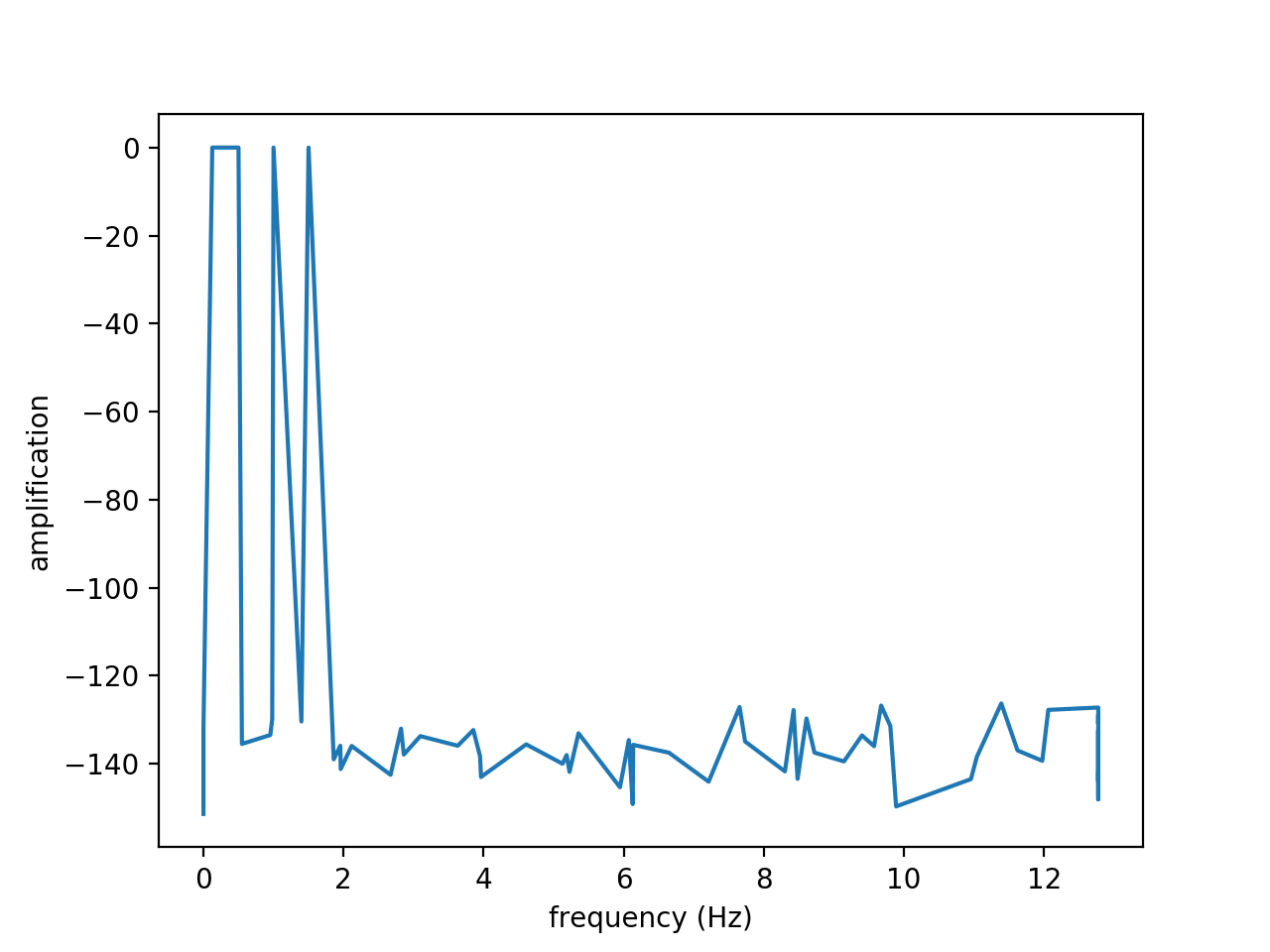
Figures above show the results obtained from the signal \(f(t)\) on the time interval \(t \in [0, 20]\) discretized with \(n=512\) time steps:
\(f(t) = 2 cos(2 \pi t) + 0.5 sin(3 \pi t) + cos(\pi t + 5) + sin(0.789 t)\)
From left to right, figures show the original and reconstructed signals (using 10 modes), the amplitude and the amplification. The amplitude exhibits four modes. Note that the amplification is close to zero as expected since the wave is neither amplified nor attenuated.
Construction
import antares
myt = antares.Treatment('dmd1d')
Parameters
- base:
Base The input base that contains one zone which contains one instant. The instant contains at least two 1-D arrays that represent a time signal.
- base:
- noiselevel: float, default= 1e-9
The noise level should be increased when ill-conditioned and non-physical modes appear.
- reconstruction_modes_number: int, default= -1
Number of modes used for the reconstruction (sorted by decreasing energy).
- type: str in [‘mod/phi’, ‘im/re’], default= ‘mod/phi’
The decomposition type of the DMD:
mod/phi for modulus/phase decomposition or
im/re for imaginery/real part decomposition.
- variables: list(str)
The variable names. The variable representing time must be the first variable in the list of variables. The other variables are the DMD variables.
- resize_time_factor: float, default= 1.0
Factor to re-dimensionalize the time variable (time used will be time_var * resize_time_factor). This is useful when you only have the iteration variable and when the time-step used is constant.
- time_t0: float, default= None
Time from which the analysis will begin.
- time_tf: float, default= None
Time to which the analysis will end.
- complex: bool, default= False
If True, the algorithm of the DMD uses complex arrays.
Preconditions
The variable representing time must be the first variable in the list of variables. The other variables are the DMD variables.
Postconditions
The treatment returns two output bases:
the first base corresponds to the DMD (spectrum in the example below)
the second base returns the input signal and the reconstructed signal for each variable.
Using the DMD algorithm, the amplitude \(||\Phi||^2\) and the amplification \(\mathbb{R}(\omega)\) of each mode are returned in the spectrum base, as well as the modulus and the phase (or the imaginary and real parts, depending on the type of DMD).
References
P. J. Schmid: Dynamic mode decomposition of numerical and experimental data. J. Fluid Mech., vol. 656, no. July 2010, pp. 5–28, 2010.
Example
import antares
myt = antares.Treatment('dmd1d')
myt['base'] = base
myt['variables'] = ['time', 'pressure', 'vx']
myt['noiselevel'] = 1e-4
myt['reconstruction_modes_number'] = 10
myt['resize_time_factor'] = 3.0E-7
myt['time_t0'] = 0.0294
myt['time_tf'] = 0.0318
spectrum, signal = myt.execute()
Main functions
Example
"""
This example illustrates the Dynamic Mode Decomposition
of a 1D signal (massflow.dat).
"""
import os

import antares

if not os.path.isdir("OUTPUT"):
    os.makedirs("OUTPUT")

# ------------------
# Reading the files
# ------------------
reader = antares.Reader("column")
reader["filename"] = os.path.join("..", "data", "1D", "massflow.dat")
base = reader.read()

# -------
# DMD 1D
# -------
treatment = antares.Treatment("Dmd1d")
treatment["base"] = base
treatment["variables"] = ["iteration", "convflux_ro"]
treatment["noiselevel"] = 1e-4
treatment["reconstruction_modes_number"] = 10
treatment["resize_time_factor"] = 3.0e-7
treatment["time_t0"] = 0.0294
treatment["time_tf"] = 0.0318
spectrum, signal = treatment.execute()

# -------------------
# Writing the result
# -------------------
writer = antares.Writer("column")
writer["base"] = spectrum
writer["filename"] = os.path.join("OUTPUT", "ex_dmd1d_spectrum.dat")
writer.dump()

writer = antares.Writer("column")
writer["base"] = signal
writer["filename"] = os.path.join("OUTPUT", "ex_dmd_signal.dat")
writer.dump()