Fast Fourier Transform (1-D signals)¶

Description¶

Computes a Fast Fourier Transform (FFT) of a signal.

Parameters¶

base: Base
The input base that contains many zones (independent to each others, typically many probes).
dtype_in: str in [‘re’, ‘mod/phi’, ‘im/re’], default= ‘re’
The decomposition type of the initial time signal: re if real signal, mod/phi or im/re if complex signal (modulus/phase or imaginery/real part decomposition respectively). If the signal is complex, a suffix must be added to the name of the variable depending on the decomposition (_im and _re for im/re, _mod and _phi for mod/phi). If given, the phase must be expressed in degrees.
dtype_out: str, default= ‘mod/phi’
The decomposition type of the output signal: mod/phi or im/re (modulus/phase or imaginery/real part decomposition respectively). If given, the phase is expressed in degrees.
resize_time_factor: float, default= 1.0
Factor to re-dimensionalize the time variable (time used will be time_var * resize_time_factor). This is useful when you only have the iteration variables and when the time-step used is constant.
time_t0: float, default= None
Time from which the analysis will start.
time_tf: float, default= None
Time to which the analysis will end.
zero_padding: float, default= 1.0
Greater than 1.0 to use zero padding in the FFT computation.

Preconditions¶

Each zone contains one Instant object. Each instant contains at least:

two 1-D arrays if the initial signal is real or
three 1-D arrays (if it is complex).

The variable representing time must be the first variable in the Instant. The second variable is the FFT variable if the signal is real. If the signal is complex, both the second and the third variables are used, and the dtype_in must be given to specify the decomposition (mod/phi or im/re). Other variables are ignored.

To change the ordering of variables, you may use base slicing.

Postconditions¶

The output base contains many zones. Each zone contains one instant. Each instant contains three 1-D arrays:

The frequencies (variable named ‘frequency’)
The FFT parts depending on the type of decomposition

Example¶

import antares
myt = antares.Treatment('fft')
myt['base'] = base
myt['dtype_out'] = 'mod/phi'
myt['resize_time_factor'] = 3.0E-7
myt['zero_padding'] = 4.0
myt['time_t0'] = 0.0294
myt['time_tf'] = 0.0318
fftbase = myt.execute()

Main functions¶

class antares.treatment.TreatmentFft.TreatmentFft¶

execute()¶

Execute the treatment.

Returns:

a base that contains many zones. Each zone contains one instant. Each instant contains three 1-D arrays:

The frequencies (variable named ‘frequency’)
The FFT parts depending on the type of decomposition

Return type:

Base

Example: real signal¶

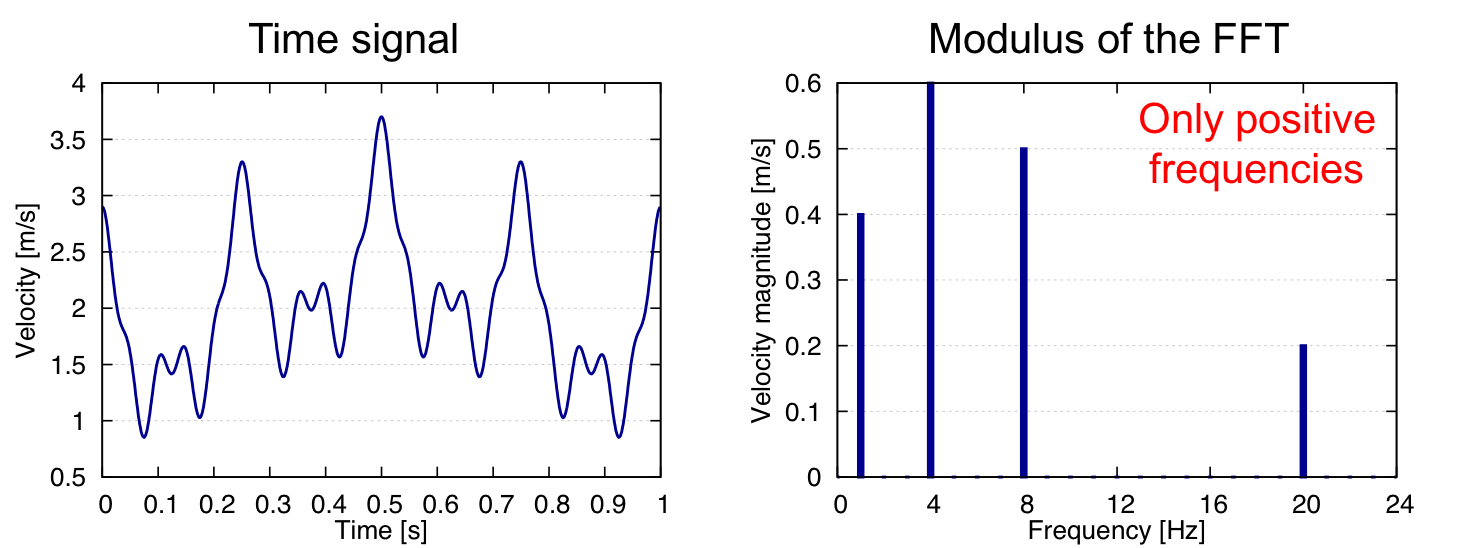
The signal is given by the following function:

Periodic case¶

Since the signal is periodic with \(t \in [0, 1]\), zero padding is not needed. The type of input data must be set to real (‘dtype_in’ = ‘re’). The base must contain two variables (t, u).

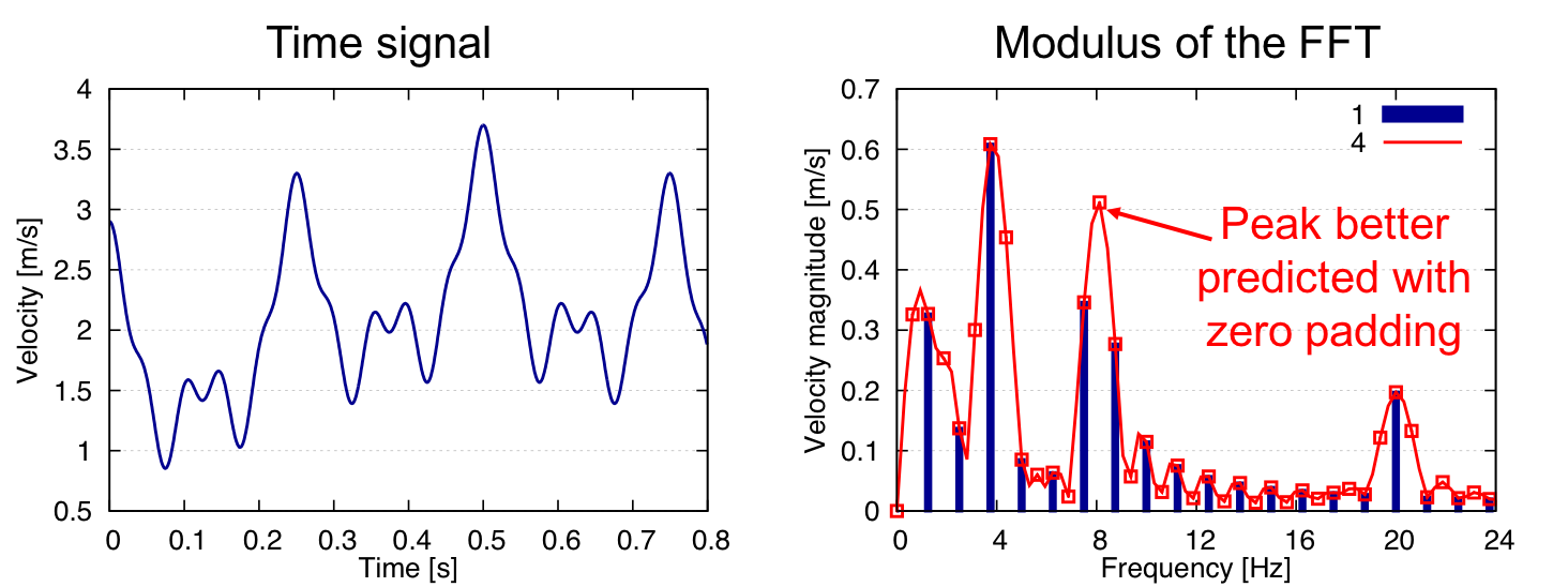
Non periodic case¶

Since the signal is not periodic with \(t \in [0, 0.8]\), zero padding can be used to have a better prediction of the peaks. Example of results for zero_padding = 1 (i.e. no zero padding) and zero_padding = 4.

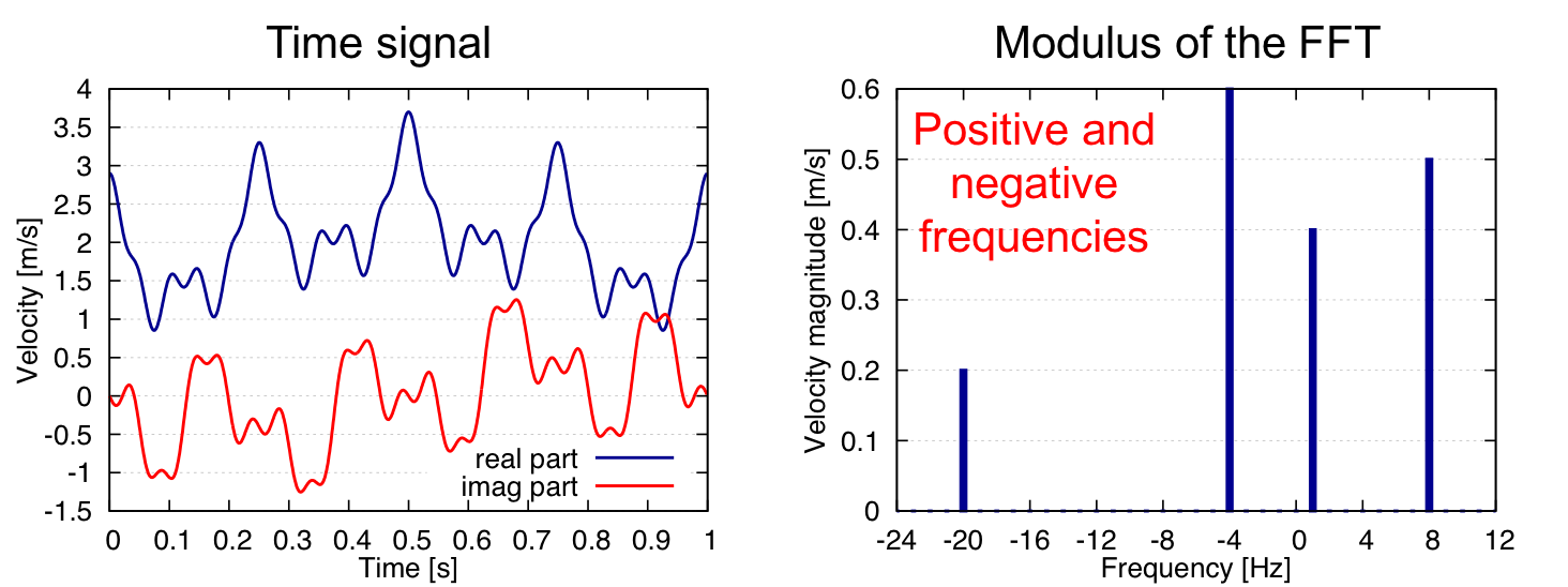
Example: complex signal¶

The signal is given by the following function:

Since the signal is periodic with \(t \in [0, 1]\), zero padding is not needed. The type of input data must be set to complex (‘dtype_in’ = ‘im/re’ or ‘mod/phi’). The base must contain three variables (t, im(u), re(u)) or (t, mod(u), phi(u)) depending on the decomposition.

Example of Application Script¶

"""
This example illustrates the Fast Fourier Transform
treatment of Antares. The signal is analyzed on a time window
corresponding to [0.0294, 0.0318] and it is zero padded

WARNING, in this case, the file read contains only two
variables, iteration and convflux_ro, the treatment use
the first one as time variable and the second as fft variable.
In case of multiple variables, the first one must be the time variable
and the second one the fft variable. To do so, use base slicing.
"""
import os
if not os.path.isdir('OUTPUT'):
    os.makedirs('OUTPUT')

from antares import Reader, Treatment

# ------------------
# Reading the files
# ------------------
reader = Reader('column')
reader['filename'] = os.path.join('..', 'data', '1D', 'massflow.dat')
base = reader.read()

# ----
# FFT
# ----
treatment = Treatment('fft')
treatment['base'] = base
treatment['dtype_out'] = 'mod/phi'
treatment['resize_time_factor'] = 3.0E-7
treatment['zero_padding'] = 4.0
treatment['time_t0'] = 0.0294
treatment['time_tf'] = 0.0318
result = treatment.execute()

# the mean of the signal can be retrieved by calling
# 'mean' attr at instant level
print('signal temporal mean:', result[0][0].attrs['convflux_ro_mean'])

# each part of the decomposition is stored as a new variable
print('result variables:', list(result[0][0].keys()))