Spectral Proper Orthogonal Decomposition

Description

This treatment computes the Spectral Proper Orthogonal Decomposition (SPOD) for a mono-zone base and for all or a subset of variables present in the base. The implementation is based on the description provided by Schmidt et al. (2020).

The SPOD computes the spatio-temporal modes of the flow. These modes are calculated as the eigenvectors of the cross-spectral density (CSD) matrix. The SPOD relies heavily on Welch’s method in which the temporal data is split into several overlapping blocks and then the DFT is computed on each block. Then, the CSD matrix for a given frequency is estimated from the frequency data of each of the DFT blocks. Finally, the modes \(\hat{\Phi}\) at each frequency corresponds to the eigenvectors of the estimation of the CSD matrix \(\hat{C}\).

\[\hat{C} W \hat{\Phi} = \hat{\Phi} \hat{\Lambda}\]

Where \(W\) is a weight matrix that can be used to take into consideration the mesh refinement or the difference in the fluctuation magnitude of the different variables, and \(\hat{\Lambda}\) are the eigenvalues containing the energy of each mode.

Parameters

• base: Base, default= None

  The input base with which the SPOD is computed. The base must contain only one zone.

• dt: float , default= None

  Time step between two instants.

• variables: list(str) , default= None

  The variables with which the SPOD is computed. If None, then the SPOD will be computed on all variables present in the base.

• volume: str, default= None

  The name of the variable containing the cell volume. If None, then the volume is computed from the base.

• nb_modes: int , default= None

  In basic mode: the desired number of modes per frequency.

• nb_frequencies: int , default= None

  In basic mode: the desired number of frequencies.

• overlap_ratio: float , default= 0.5

  In basic mode: the overlapping ratio between two DFT blocks.

• nb_instants_per_block: int, default= None

  In advanced mode: the number of instants per DFT block.

• nb_overlap: int, default= None

  In advanced mode: the number of overlapping instants in the DFT blocks.

• nb_zero_padding: int, default= None

  In advanced mode: the number of zeros added to the DFT blocks.

• norm: str , default= ‘identity’

  The normalization matrix \(W\):

  • 'identity': no normalization (\(W=I\)).

  • 'volume': normalize by the cell volume.

  • 'turbulent_kinetic_energy': normalize by the turbulent kinetic energy (variables must be the velocity vector components).

  • 'total_energy_ruvwt': normalize by the total energy when the variables are density, velocity and temperature.

  • 'total_energy_puvws': normalize by the total energy when the variables are pressure, velocity and entropy.

  • 'acoustic_energy': normalize by the acoustic energy when the variables are density and velocity.

  Warning

  Some normalization functions require a specific order in the variables keywords and/or the definition of extra parameters. See the normalization section for further details on how to use the different options available.

• window_type: str or callable , default= ‘hamming’

  The window used in the DFT. The user can pick between the following predefined windows: 'uniform', 'hanning', 'blackman', 'hamming', and 'bartlett'.

  If none of the above suits you, you can also set your own custom window function. The window function must be a function that accepts an integer \(N\) representing the length of the unpadded block signal, and returns a single array of length \(N\) with the window data.

  Example : The following code defines a triangular window using the function triang in the scipy.signal library

  import scipy.signal
  
  def my_triangular_window(N):
      return scipy.signal.triang(N)
  
  tt = antares.Treatment('spod')
  tt['window_type'] = my_triangular_window
  

• confidence_lvl: float , default= None

  The confidence interval for the energy modes.

• mean_type: str , default= ‘long-term’

  The type of mean subtracted to the DFT blocks:

  • 'long-term': subtract the mean of the entire base.

  • 'blockwise': subtract only the mean of the corresponding block.

• rho: str or float , default= None

  The string containing the name of the density variable or a float value if it is assumed to be constant.

• gamma: str or float , default= None

  The string containing the name of the specific heat ratio capacity variable or a float value if it is assumed to be constant.

• R: str or float , default= None

  The string containing the name of the mass specific gas constant variable or a float value if it is assumed to be constant.

• speed_of_sound: str or float, default= None

  The string containing the name of the speed of sound variable or a float value if it is assumed to be constant.

• output_modes: bool , default= False

  If True, the treatment will output 2 bases, the first will contain the energy of the modes and the second will contain the spatial modes. If False, only the modes energy is output.

• large_data_directory: str , default= None

  If not None, intermediary results will be saved in this directory to decrease the memory footprint.

• filter_output_frequencies: list(list or float), default= None

  If None, compute the SPOD modes for all frequencies.

  Otherwise, compute the SPOD modes only for specific frequencies. The syntax is a list whose elements can be:

  • A single number \(n\): Compute the modes for the nearest frequency to \(n\)

  • A list of the form [a, b]: Compute the modes for all frequencies \(f\) in the range \(a \le f \le b\)

  Example 2 shows the usage of this keyword.

• frequencies_as_instants: bool, default= False

  If True, the output modes base will be formatted as base[variable][frequency][mode].

  If False, the output modes base will be formatted as base[variable][mode][frequency].

• compute: str , default= ‘full’

  • 'full': compute both the DFT and SPOD

  • 'dft': compute only the DFT part and save the result in large_data_directory

  • 'spod': read the DFT results in large_data_directory and compute the SPOD part

Preconditions

The following conditions must be met in order to ensure a correct execution of the treatment:

• The input base must be unstructured

• The input base must contain only one zone.

• The input base must be either 2D or 3D dimensional.

• All the instants must contain the variables specified in the variables keyword and any other extra variable related to the normalization

Postconditions

If output_modes = False, the treatment outputs one base containing the energy of each mode. This base contains one zone, and 1 or 3 instants called ‘modes’, ‘confidence_lower’, and ‘confidence_upper’. The last two instants are present only if confidence_lvl is not None. Each of these instants contains a variable called ‘frequency’ with all the frequencies computed and several instants called ‘mode_xxx’ containing the energy per frequency of each mode, and the lower or upper end of the confidence intervals. The modes are sorted such as ‘mode_000’ is the most energetic mode, ‘mode_001’ is the second most energetic mode, and so on.

If output_modes = True, the treatment outputs a list of two bases. The first base is the energy base described above. The second base contains the SPOD modes. This base has as many zones as variables on which the SPOD was computed (similarly to the previous base, the modes are sorted by energy). The instants in each zone will be formatted according the frequencies_as_instants keyword.

Basic and advanced modes

This treatment can be used in “basic” or “advanced” mode. In the “basic” mode, the user specifies the number of desired modes and frequencies in the output, as well as the overlap ratio between the DFT blocks. The treatment will internally compute how the database should be divided and zero-padded to satisfy these conditions. In the “advanced” mode, the user selects the number of instant per DFT blocks, the number of overlapping instants between the block and the number of zeros padded to each DFT block. The number of modes and frequencies will, therefore, be determined by these choices. The keywords to specify for each mode are the following:

• Basic mode keywords:

  • nb_modes

  • nb_frequencies

  • overlap_ratio (optional)

• Advanced mode keywords:

  • nb_instants_per_block

  • nb_overlap

  • nb_zero_padding

Warning

Only one set of keys should be specified for the treatment to work. Simultaneously setting “basic” and “advanced” keywords will lead to an error when executing the treatment.

Normalizations

• ‘identity’

\[W = I\]

• ‘volume’

\[W = \int_{V} dV\]

• ‘turbulent_kinetic_energy’

If variables is set to the velocity components u, v, w, then we can normalize by the turbulent kinetic energy (TKE). In this case, the weight matrix is given by:

\begin{equation} W =\int_{V} \left[\begin{array}{ccc} 1\\ & 1\\ & & 1 \end{array}\right]dV \end{equation}

• ‘total_energy_ruvwt’

If variables is set to the density, velocity components and temperature (in that order), then we can normalize by the total energy. In this case, the weight matrix is given by:

\begin{equation} W = \int_{V} \left[\begin{array}{ccccc} \frac{\overline{a_0}^2}{\overline{\gamma} \; \overline{\rho}} \\ & \overline{\rho} \\ & & \overline{\rho} \\ & & & \overline{\rho} \\ & & & & \frac{ \overline{\rho} \overline{R} }{(\overline{\gamma} - 1) \overline{T}} \end{array}\right]dV \end{equation}

In order to use this normalization the following keywords must be specified: gamma, R, and speed_of_sound

• ‘total_energy_puvws’

If variables is set to the pressure, velocity components and entropy (in that order), then we can normalize by the total energy. In this case, the weight matrix is given by:

\begin{equation} W = \int_{V} \left[\begin{array}{ccccc} \frac{\overline{\rho} \; \overline{a_0}^2}{\overline{\gamma}^2 \; \overline{P}^2} \\ & \overline{\rho} \\ & & \overline{\rho} \\ & & & \overline{\rho} \\ & & & & \frac{( \overline{\gamma} - 1) \overline{P} }{\overline{\gamma} \overline{R}^2} \end{array}\right]dV \end{equation}

In order to use this normalization the following keywords must be specified: gamma, R, speed_of_sound, and rho

• ‘acoustic_energy’

If variables is set to the density, velocity components and temperature (in that order), then we can normalize by the total energy. In this case, the weight matrix is given by:

\begin{equation} W = \int_{V} \left[\begin{array}{cccc} \frac{\overline{a_0}^2}{\overline{\gamma} \; \overline{\rho}} \\ & \overline{\rho} \\ & & \overline{\rho} \\ & & & \overline{\rho} \\ \end{array}\right]dV \end{equation}

In order to use this normalization the following keywords must be specified: gamma, and speed_of_sound

Validation

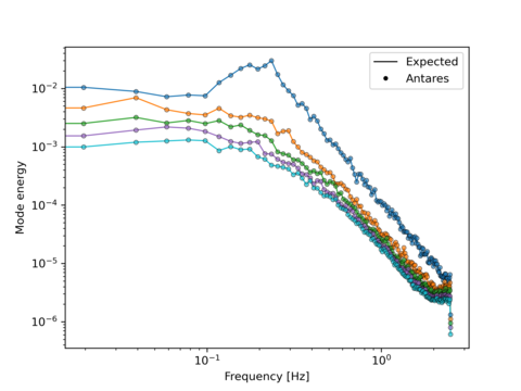
This treatment was validated comparing the results to 4 different publicly available SPOD implementations, one done in MATLAB and another in Python.

These test cases correspond to:

• 2D subsonic jet flow (Brès et al. 2018)

• Flow over 2D Backward facing step (He et al. 2022)

• Pressure field over a compressor blade (He et al. 2022)

• 2D turbine cooling film (Wang et al. 2021)

As an example, we show below the comparison between the first 5 expected modes energy and the energy obtained using the treatment for the first test case:

Main functions

class antares.treatment.TreatmentSPOD.TreatmentSPOD

execute()

Example 1: SPOD treatment in basic mode without normalization

The following example computes the SPOD on a 2D jet flow example. The data corresponds to LES simulation of a subsonic jet at \(Ma=0.9\) (Brès et al. 2018). The original database can be found here. The simulation domain is a 2D rectangle with a structured mesh with a refinement in the jet zone. The database is composed of the pressure field for 5000 timesteps (\(\Delta t = 0.2\)). The mesh and an animation of the pressure profile is shown below.

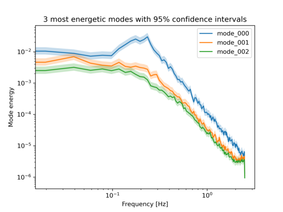
The script below computes 38 SPOD modes with 128 frequencies per mode for this configuration. The DFT blocks are split so there is a 50% overlap, as we use the hamming window function. For this case, no normalization is used the 95% confidence intervals are calculated for the each mode energy. We, additionally, show a post-processing example to plot the energy of the 3 most energetic modes along with their confidence intervals. Finally, we output the modes for future visualization.

"""
Example of SPOD treatment in basic mode

to run:
python spod_basic.py
"""

import os
import antares
import matplotlib.pyplot as plt

data_folder = os.path.join('..', 'data', 'SPOD')
output_folder = os.path.join(data_folder, 'OUTPUT')
output_modes_folder = os.path.join(output_folder, 'modes')
os.makedirs(output_folder, exist_ok=True)
os.makedirs(output_modes_folder, exist_ok=True)

# Read 2D jet data
# ----------------
reader = antares.Reader('bin_tp')
reader['filename'] = os.path.join(data_folder, '2D_jet', 'jet<instant>.plt')
jet_data = reader.read()

# Check if the base is structured:
if jet_data.is_structured():
    jet_data.unstructure()

# Apply SPOD treatment
# --------------------
spod = antares.Treatment('spod')
spod['base'] = jet_data
spod['variables'] = ['pressure']
spod['nb_modes'] = 38
spod['nb_frequencies'] = 128
spod['overlap_ratio'] = 0.5
spod['dt'] = 0.2
spod['window_type'] = 'hamming'
spod['norm'] = 'identity'
spod['confidence_lvl'] = 0.95
spod['output_modes'] = True
spod['frequencies_as_instants'] = True
energy_base, spod_modes = spod.execute()

# Plot the energy for the 3 most energetic modes
# ----------------------------------------------

for idx in range(3):
    freq = energy_base[0]['modes']['frequency']
    energy = energy_base[0]['modes'][f'mode_{idx:03d}']
    conf_lower = energy_base[0]['confidence_lower'][f'mode_{idx:03d}']
    conf_upper = energy_base[0]['confidence_upper'][f'mode_{idx:03d}']

    plt.loglog(freq, energy, label = f'mode_{idx:03d}')
    plt.fill_between(freq, conf_lower, conf_upper, alpha=0.25)

plt.xlabel('Frequency [Hz]')
plt.ylabel('Mode energy')
plt.title('3 most energetic modes with 95% confidence intervals')
plt.legend()
plt.savefig(os.path.join(output_folder, 'spod_jet_mode_energies.png'), dpi=300)

# Save the spatial modes for visualization
# ----------------------------------------

writer = antares.Writer('hdf_antares')
writer['base'] = spod_modes
writer['filename'] = os.path.join(output_modes_folder, 'modes')
writer.dump()

The 3 most energetic modes with 95% confidence are shown below:

Example of visualization of two of the modes at two different frequencies:

• First mode at \(f=0.0585\) Hz

• Fifth mode at \(f=0.683\) Hz

Example 2: SPOD Treatment in advanced mode with total energy normalization

The following example computes the SPOD on a 2D film cooling flow DDES simulation (Wang et al. 2021). The simulation domain is a 2D slice of the mixing between the coolant and the hot stream. The database contains the density, velocity, temperature and the speed of sound.

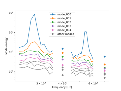
The script below shows how to use the advanced mode of the SPOD treatment. The database is divided into blocks of 128 points, with a 64 points overlap between blocks and no zero padding. The SPOD is normalized using the total energy (‘total_energy_ruvwt’). Additionally, we only compute the SPOD modes for the frequencies between 2200Hz-3500Hz, 4500Hz-6000Hz, and for the frequency closest to 4010Hz and 7000Hz. Finally, the energy of all modes for the aforementioned frequency ranges is plotted in a single figure.

"""
Example of SPOD treatment in advanced mode

to run:
python spod_advanced.py
"""

import os
import antares
import matplotlib.pyplot as plt
import numpy as np

data_folder = os.path.join('..', 'data', 'SPOD')
output_folder = os.path.join(data_folder, 'OUTPUT')
output_modes_folder = os.path.join(output_folder, 'modes')
os.makedirs(output_folder, exist_ok=True)
os.makedirs(output_modes_folder, exist_ok=True)

# Read data
# ----------------
reader = antares.Reader('bin_tp')
reader['filename'] = os.path.join(data_folder, 'Turbine_film_cooling', 'cooling_<instant>.plt')
data = reader.read()

# Check if the base is structured:
if data.is_structured():
    data.unstructure()

## Setup and run treatment
spod = antares.Treatment('spod')
spod['base'] = data
spod['variables'] = ['rho', 'u', 'v', 'T']
spod['nb_instants_per_block'] = 128
spod['nb_overlap'] = 64
spod['nb_zero_padding'] = 0
spod['dt'] = 6.25e-5
spod['window_type'] = 'hamming'
spod['norm'] = 'total_energy_ruvwt'
spod['gamma'] = 1.4
spod['R'] = 287
spod['speed_of_sound'] = 'speed_of_sound'
spod['output_modes'] = False
spod['filter_output_frequencies'] = [[2200, 3500], [4500, 6000], 4010, 7000]
spod['volume'] = 'volume'
energy_base = spod.execute()

# Plot the 5 most energetic modes with different colors
legend_lines = []
colored_modes = 5
mode_colors = ['tab:blue', 'tab:orange', 'tab:green', 'tab:purple', 'tab:pink']
for idx in range(colored_modes):
    for rdx, f in enumerate(spod['filter_output_frequencies']):
        if type(f) is list:
            mask = (f[0] <= energy_base[0]['modes']['frequency']) & \
                   (energy_base[0]['modes']['frequency'] <= f[1])
        else:
            f_idx = (np.abs(f - energy_base[0]['modes']['frequency'])).argmin()
            mask = [False for _ in range(len(energy_base[0]['modes']['frequency']))]
            mask[f_idx] = True

        freq = energy_base[0]['modes']['frequency'][mask]
        energy = energy_base[0]['modes'][f'mode_{idx:03d}'][mask]
        if sum(mask) == 1:
            l = plt.loglog(freq, energy, label = f'mode_{idx:03d}', color=mode_colors[idx], linestyle='-', marker='o')
        else:
            l = plt.loglog(freq, energy, label = f'mode_{idx:03d}', color=mode_colors[idx], linestyle='-', marker='')
    legend_lines.append(l[0])


# Plot the remaining modes in grey
for idx in range(colored_modes, len(energy_base[0][0].keys())-1):
    for rdx, f in enumerate(spod['filter_output_frequencies']):
        if type(f) is list:
            mask = (f[0] <= energy_base[0]['modes']['frequency']) & \
                   (energy_base[0]['modes']['frequency'] <= f[1])
        else:
            f_idx = (np.abs(f - energy_base[0]['modes']['frequency'])).argmin()
            mask = [False for _ in range(len(energy_base[0]['modes']['frequency']))]
            mask[f_idx] = True

        freq = energy_base[0]['modes']['frequency'][mask]
        energy = energy_base[0]['modes'][f'mode_{idx:03d}'][mask]
        if sum(mask) == 1:
            l = plt.loglog(freq, energy, label = f'other modes', color='tab:grey', linestyle='-', marker='o')
        else:
            l = plt.loglog(freq, energy, label = f'other modes', color='tab:grey', linestyle='-', marker='')

legend_lines.append(l[0])

plt.xlabel('Frequency [Hz]')
plt.ylabel('Mode energy')
plt.legend(handles=legend_lines)
plt.savefig(os.path.join(output_folder, 'spod_cooling_mode_energies.png'), dpi=300)

References

G. A. Brès, P. Jordan, M. Le Rallic, V. Jaunet, A. V. G. Cavalieri, A. Towne, S. K. Lele, T. Colonius, O. T. Schmidt, (2018). Importance of the nozzle-exit boundary-layer state in subsonic turbulent jets, Journal of Fluid Mechanics 851, 83-124. (link).

He, X., Zhao, F., and Vahdati, M. (2022). Detached Eddy Simulation: Recent Development and Application to Compressor Tip Leakage Flow. ASME. Journal of Turbomachinery 144(1): 011009. (link).

Schmidt, O. T., Towne, A., Rigas, G., Colonius, T., & Bres, G. A. (2018). Spectral analysis of jet turbulence. Journal of Fluid Mechanics, 855, 953-982. (link).

Schmidt, O. T., & Colonius, T. (2020). Guide to spectral proper orthogonal decomposition. AIAA journal, 58(3), 1023-1033. (link).

Sieber, M., Paschereit, C. O., & Oberleithner, K. (2016). Spectral proper orthogonal decomposition. Journal of Fluid Mechanics, 792, 798-828. (link)

Wang, R., & Yan, X. (2021). Delayed-detached eddy simulations of film cooling effect on trailing edge cutback with land extensions. ASME Journal of Engineering for Gas Turbines and Power, 143(11), 111004. (link)

Link to MATLAB implementation repository

Link to Python implementation repository