
Error
This treatment is provided by an external module and is not part of the core system. If you’re interested in accessing or utilizing this feature, please contact us for further details and support.
Wake Acoustic
Description
Analyse the wake turbulence on a structured revolution surface around the axis of a turbomachine.
The turbulence of the flow is assumed to be modelled by the \(k-\varepsilon\), \(k-\omega\) or \(k-l\) (Smith) models.
The analysis provided by the treatment is a set of radial profiles of values of interest: a set of variables defined by the user, plus \(urms\) (turbulent velocity), \(Lint_1\) (integral length scale estimated through a gaussian fit of the wake), \(Lint_2\) (integral length scale estimated through turbulent variables), \(C\) and \(L\) (coefficients used to define \(Lint_2\)).
Different analyses are possible depending on the needs of the user:
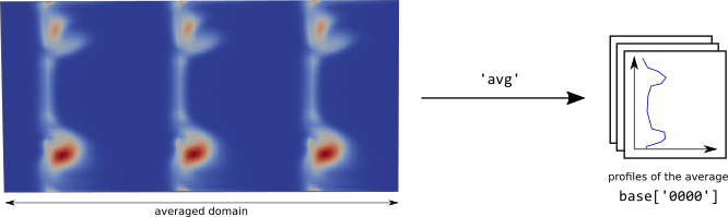
avg: azimuthal average of values of interest at each radius.
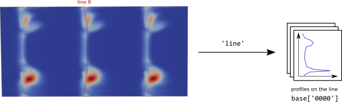
line: extraction of values of interest on a line \(\theta(r)\) defined by the user.
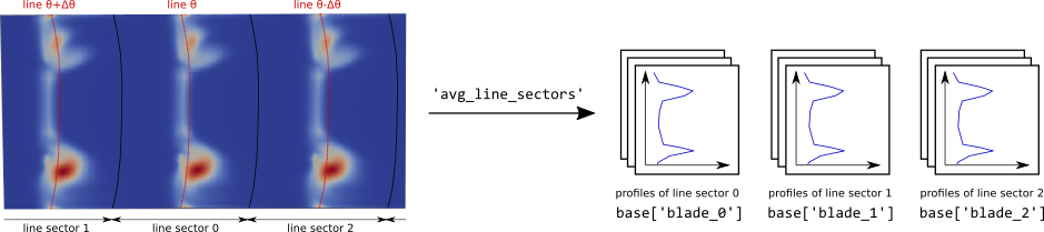
avg_line_sectors: azimuthal average of values of interest over sectors centered on a \(\theta(r)\) line.
avg_wake_sectors: azimuthal average of values of interest over sectors centered on the center of wakes.

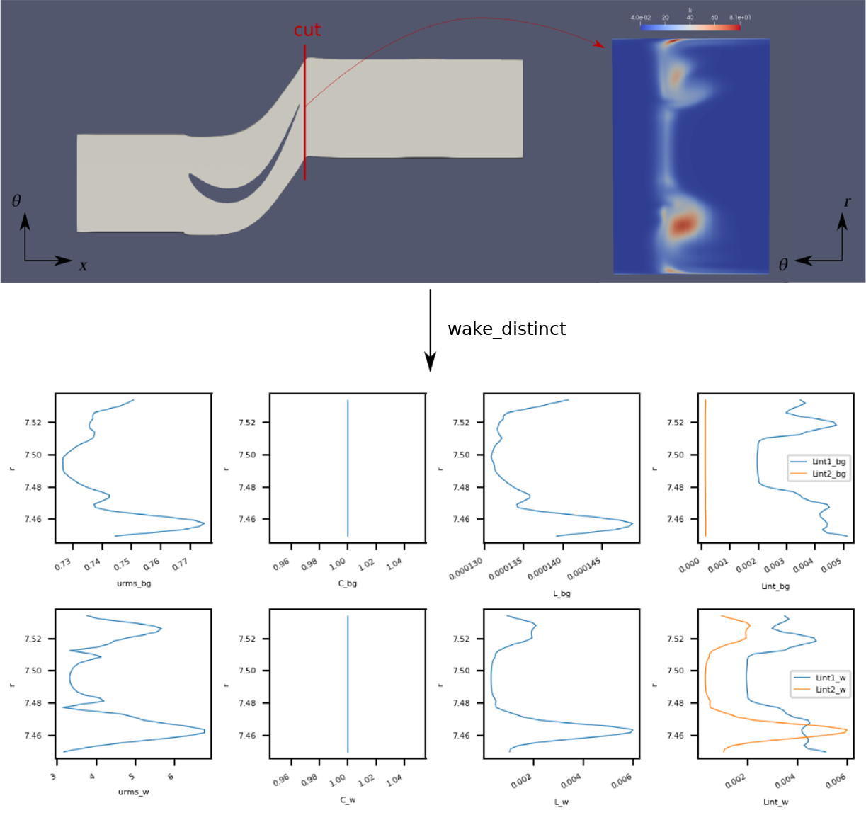
wake_distinct: extraction of values over sectors centered on the center of wakes with wake gaussian modeling.
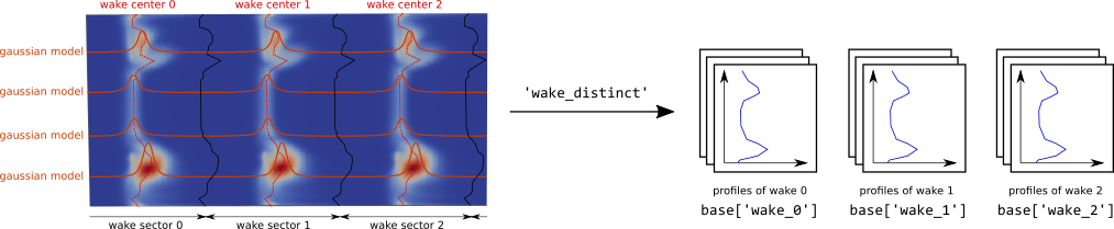
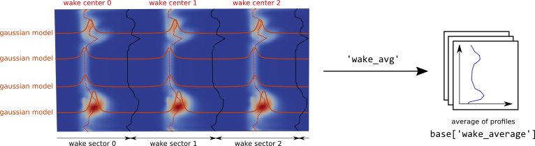
wake_avg: average over sectors of profiles of wake_distinct.
These analyses and the formulae used are documented in the Formulae section.
Parameters
- base:
Base The input base on which the wake is analysed. Read section Preconditions to know the assumptions on this base.
- base:
- cylindrical_coordinates:
list(str), default= [‘x’, ‘r’, ‘theta’] Names of the cylindrical coordinates: the axis of rotation (axial coordinate), the distance to this axis (radius), and the azimuth.
- cylindrical_coordinates:
- type:
str Type of analysis to perform (possibilities are avg, line, avg_line_sectors, avg_wake_sectors, wake_distinct and wake_avg).
- type:
- turbulence_model:
list(str) Name of the turbulence model used (possibilities are k-epsilon, k-omega and k-l).
- turbulence_model:
- turbulence_variables:
list(str) Name of the turbulence variables, e.g. [‘k’, ‘l’].
- turbulence_variables:
- coef_variable:
str, default= None Name of the coefficient \(C\) used to compute \(Lint2\). When None, the default formulation given in subsection Extra Formulae is used, otherwise the formulation given in the computer model of the base is used (optional).
- coef_variable:
- static_temp_variable:
str, default= None Name of the static temperature variable, used to compute the default formulation of \(C\) (optional when coef_variable is not None).
- static_temp_variable:
- avg_variables:
list(str), default= [] Name of the variables to average (called \(user\_variable\) in section Formulae). (optional).
- avg_variables:
- nb_azimuthal_sector:
int The input base is considered as one azimuthal sector. This parameter is the number of azimuthal sectors needed to fill a 360 deg configuration (e.g. when the base is 360 deg, nb_azimuthal_sector has value 1, when base is < 360 deg, nb_azimuthal_sector has value more than 1). (optional when using avg analysis).
- nb_azimuthal_sector:
- nb_blade:
int Number of blades per azimuthal sector. (optional when using avg and line analyses).
- nb_blade:
- line_base:
Base The base representing the line \(\theta(r)\). (optional: only for line and avg_line_sectors analyses).
- line_base:
- wake_factor:
float A percentage (in [0, 1]) used for wake analysis. (optional: only for wake_distinct and wake_avg analyses).
- wake_factor:
- wake_detection:
strortuple(str,str), default= ‘urms’ The physical quantity that is used to detect the wake. The gaussian fit is applied on this quantity. The quantity must be among ‘V’, ‘Vx’, ‘tke’, or ‘urms’.
If wake_detection is a tuple, the first string of the tuple must be among ‘V’, ‘Vx’, or ‘tke’. The second string is the variable name found in the input base. ‘V’ is the magnitude of the velocity. ‘Vx’ is the axial component of the velocity vector. ‘tke’ is the turbulent kinetic energy.
If the tuple notation is not used, then the variable in the input base must be among ‘V’, ‘Vx’, or ‘tke’. The variables urms is always computed in the treatment.
(optional: only for wake_distinct and wake_avg analyses).
- wake_detection:
- option_X_bg:
str, default= avg Option for background variables formulation, see Extra Formulae. (optional: only for wake_distinct and wake_avg analyses).
- option_X_bg:
- option_X_w:
str, default= avg Option for wake variables formulation, see Extra Formulae. (optional: only for wake_distinct and wake_avg analyses).
- option_X_w:
Preconditions
The base must be 2D, and periodic in azimuth. The base must fulfill the following hypotheses: structured, monozone, shared radius and azimuth, regularity in r and theta (i.e. it is a set of rectangular cells in cylindrical coordinates), r is the first dimension and theta is the second dimension of the surface.
The base can be multi-instant.
The line_base must be 1D. If the line_base does not fulfill the following assumptions, the line_base is “normalized”: structured, monozone, shared radius, radius values sorted strictly ascending.
The line_base must be mono-instant.
Postconditions
New variables are added to the input base.
The output base contains one zone per set of profiles.
Example
# construction of a 2D base fulfilling the assumptions (see Preconditions).
# with cylindrical coordinates: 'x', 'r', 'theta'
# using k-epsilon turbulence model, with turbulent variables: 'k', 'eps'
# representing 1 over 22 azimuthal sectors, with 2 blades per azimuthal sector

b.set_formula('C = 1.0') # user-defined C coefficient (chosen arbitrarily in this example)

t = Treatment('wakeacoustic')
t['base'] = b
t['cylindrical_coordinates'] = ['x', 'r', 'theta']
t['type'] = 'avg_wake_sectors'
t['turbulence_model'] = 'k-epsilon'
t['turbulence_variables'] = ['k', 'eps']
t['coef_variable'] = 'C'
t['nb_azimuthal_sector'] = 22
t['nb_blade'] = 2
base_out = t.execute()

# plot profiles
# e.g. urms_bg profile with base_out['wake_0'].shared['r'], base_out['wake_0'][0]['urms_bg']
Known limitations
For the moment, the wake centers are only computed on the first Instant, and then, multi-instant bases are not correctly handled for avg_wake_sectors, wake_distinct, wake_avg. analyses.
Formulae
Definition of the Profiles
- avg
\(user\_variable(r) = \text{mean}_\theta(user\_variable(r, \theta))\)
\(urms_{bg}(r) = \sqrt{\text{mean}_\theta(urms^2(r, \theta))}\)
\(urms_{w}(r) = 0\)
\(Lint1_{bg}(r) = \texttt{NaN}\)
\(Lint1_{w}(r) = \texttt{NaN}\)
\(C_{bg}(r) = \text{mean}_\theta(C(r, \theta))\)
\(C_{w}(r) = \text{mean}_\theta(C(r, \theta))\)
\(L_{bg}(r) = \text{mean}_\theta(L(r, \theta))\)
\(L_{w}(r) = \text{mean}_\theta(L(r, \theta))\)
\(Lint2_{bg}(r) = \text{mean}_\theta(Lint2(r, \theta))\)
\(Lint2_{w}(r) = \text{mean}_\theta(Lint2(r, \theta))\)
- line
In these formulae, \(\theta(r)\) is a user-defined line as \(line\_base\).
\(user\_variable(r) = \text{mean}_\theta(user\_variable(r, \theta))\)
\(urms_{bg}(r) = \sqrt{\text{mean}_\theta(urms^2(r, \theta))}\)
\(urms_{w}(r) = 0\)
\(Lint1_{bg}(r) = \texttt{NaN}\)
\(Lint1_{w}(r) = \texttt{NaN}\)
\(C_{bg}(r) = C(r, \theta(r))\)
\(C_{w}(r) = C(r, \theta(r))\)
\(L_{bg}(r) = L(r, \theta(r))\)
\(L_{w}(r) = L(r, \theta(r))\)
\(Lint2_{bg}(r) = Lint2(r, \theta(r))\)
\(Lint2_{w}(r) = Lint2(r, \theta(r))\)
avg_line_sectors
Same formulae than avg, but the treatment generates one set of profiles per blade, on sectors centered on \(\theta(r) + k \cdot \Delta \theta\) of azimuthal width \(\Delta \theta = \frac{2 \pi}{nb\_azimuthal\_sector \cdot nb\_blade}\), where \(\theta(r)\) is given by the user as \(line\_base\), \(k \in \{ 0, \cdots, nb\_blade\}\).
avg_wake_sectors
Same formulae than avg, but the treatment generates one set of profiles per blade, on sectors centered on \(\theta(r, k)\) of azimuthal width \(\Delta \theta = \frac{2 \pi}{nb\_azimuthal\_sector \cdot nb\_blade}\), where \(\theta(r, k)\) is the center of the wake \(k\) at radius \(r\), \(k \in \{ 0, \cdots, nb\_blade\}\).
- wake_distinct
In these formulae, the set of \(\theta\) is the subset of all azimuthal values of the current wake \(k\).
\(user\_variable(k, r) = \text{mean}_\theta(user\_variable(r, \theta))\)
\(urms_{bg}(k, r) = \sqrt{\text{min}_\theta(urms^2(r, \theta))}\) when existing wake, otherwise \(\sqrt{\text{mean}_\theta(urms^2(r, \theta))}\)
\(urms_{w}(k, r) = a1\), given by the gaussian model when existing wake, otherwise \(0\)
\(Lint1_{bg}(k, r) = 0.21 \cdot \sqrt{\log{2}} \cdot a3 \cdot r\), where \(a3\) is given by the gaussian model when existing wake, otherwise \(\texttt{NaN}\)
\(Lint1_{w}(k, r) = 0.21 \cdot \sqrt{\log{2}} \cdot a3 \cdot r\), where \(a3\) is given by the gaussian model when existing wake, otherwise \(\texttt{NaN}\)
- \(X_{bg}(k, r)\) with \(X \in \{C, L, Lint2\}\):
if option_X_bg = ‘avg’ and existing wake, then \(X_{bg}(k, r) = \text{mean}_{\theta bg}(X(r, \theta))\)
if option_X_bg = ‘min’` and existing wake, then \(X_{bg}(k, r) = \min_{\theta bg}(X(r, \theta))\)
if wake does not exist, \(X_{bg}(k, r) = \text{mean}_{\theta}(X(r, \theta))\)
- \(X_{w}(k, r)\) with \(X \in \{C, L, Lint2\}\):
if option_X_w = ‘avg’ and existing wake, then \(X_{w}(k, r) = \text{mean}_{\theta w}(X(r, \theta))\)
if option_X_w = ‘k_max’ and existing wake, then \(X_{w}(k, r) = X(r, \text{argmax}_\theta(urms^2))\)
if option_X_w = ‘gaussian_center’ and existing wake, then \(X_{w}(k, r) = X(r, a2)\)
if wake does not exist, \(X_{w}(k, r) = \text{mean}_{\theta}(X(r, \theta))\)
where \(\theta w\) is the set of \(\theta\) such that \(\sqrt{urms^2 - \min_\theta(urms^2)} > wake\_factor \cdot \sqrt{\min_\theta(urms^2)}\), and \(\theta bg\) is its complement. Note that extracting values at \(\text{argmax}_\theta(urms^2)\), i.e. using option_X_w = ‘gaussian_center’, can lead to discontinuities in the profiles, e.g. when \(urms^2(\theta)\) has a “M”-shape near its maximum.
- wake_avg
Average of profiles of wake_avg: \(X(r) = \dfrac{1}{N} \sum\limits_{k=0}^{N-1} X(k, r)\).
Gaussian Modelling
When using analyses wake_distinct and wake_avg, the wake is modelled at each radius by a gaussian function, enabling the computation of new values of interest (in particular \(Lint1\)).
This modelling is conditionned by the wake existence, which is fulfilled when there exists \(\theta\) such that \(urms\_env (\theta) > wake\_factor \cdot \sqrt{\min_\theta(urms^2)}\), where \(urms\_env = \sqrt{urms^2 - \min_\theta(urms^2)}\).
When the wake exists, \(urms\_env\) is fitted to the gaussian function \(g(\theta) = a_1 \cdot e^{-{\left(\dfrac{\theta - a_2}{a_3}\right)}^2}\), parameterized by \(a_1\), \(a_2\) and \(a_3\), using a nonlinear least squares method.
Extra Formulae
The variables \(urms\), \(C\) and \(L\) are computed using the following relations, where \(k\), \(\varepsilon\), \(\omega\) and \(l\) are the turbulent variables:
\(urms^2 = \frac{2}{3} k\).
\(Lint2 = C \cdot L\)
\(L = \dfrac{k^{3/2}}{\varepsilon} = \dfrac{\sqrt{k}}{0.09 \cdot \omega} = \dfrac{l}{0.0848^{3/4}}\).
\(C = 0.43 + \dfrac{14}{Re_\lambda^1.05}\) or \(C\) is user-defined using base.set_formula.
\(Re_\lambda = \sqrt{\frac{20}{3} Re_L}\).
\(Re_L = \dfrac{k^2}{\varepsilon \cdot \nu} = \dfrac{k}{0.09 \cdot \omega \cdot \nu} = \dfrac{l \cdot \sqrt{k}}{0.0848^{0.75} \cdot \nu}\).
\(\nu = c_0 + c_1 \cdot T + c_2 \cdot T^2 + c_3 \cdot T^3\) (air kinematic viscosity), \(c_0 = -3.400747 \cdot 10^{-6}\), \(c_1 = 3.452139 \cdot 10^{-8}\), \(c_2 = 1.00881778 \cdot 10^{-10}\) and \(c_3 = -1.363528 \cdot 10^{-14}\).