# Reading boundary data in a HDF-CGNS file

This tutorial shows how to:

• read a turbomachinery configuration stored in HDF-CGNS format

• compute the h/H variable

• get the base corresponding to the blade given as a family

• perform node-to-cell and cell-to-node on this latter base

• make profile at some heights of the blade

• output all curves in a single HDF-CGNS file

## Reading data

If we have a mesh file mesh.cgns and a solution file elsAoutput.cgns, then we can use the Antares reader hdf_cgns.

reader = antares.Reader('hdf_cgns')
reader['filename'] = 'mesh.cgns'
reader['shared'] = True
base = reader.read()

We put the mesh as shared variables.

reader = antares.Reader('hdf_cgns')
reader['base'] = base
reader['filename'] = 'elsAoutput.cgns'
base = reader.read()

We append the solution to the previous base.

## Computing h/H variable

The letter h means the hub, and the letter H the shroud. The h/H variable is the distance of a point from the hub on a line going from the hub to the shroud.

tr = antares.Treatment('hH')
tr['base'] = base
tr['row_name'] = 'ROW'
tr['extension'] = 0.1
tr['coordinates'] = ['CoordinateX', 'CoordinateY', 'CoordinateZ']
base = tr.execute()

The option ‘row_name’ tells the convention used to prefix the names of rows in the configuration. The option ‘extension’ is 10% of the radius of the configuration.

## Get the family base

Next, we extract the blade given by the family ROW(1)_BLADE(1)

row_1_blade_1 = base[base.families['ROW(1)_BLADE(1)']]

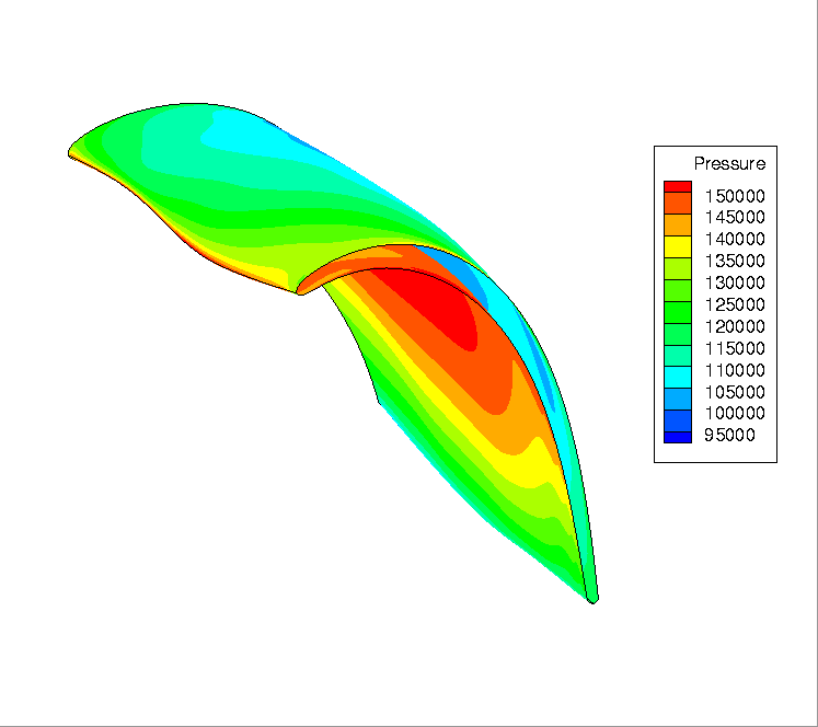
The pressure is stored in BC_t node of the HDF-CGNS file.

## Perform node-to-cell and cell-to-node on this latter base

The base row_1_blade_1 is a 2D base on which we can perform node2cell and cell2node operations.

row_1_blade_1.node_to_cell(variables=['ro'])

row_1_blade_1.cell_to_node(variables=['Pressure', 'Temperature'])

Then, we save the base in a HDF-CGNS file.

writer = antares.Writer('hdf_cgns')
writer['base'] = row_1_blade_1
writer['filename'] = 'all_wall_row_1_blade_1.cgns'
writer['base_name'] = 'row_1_blade_1'
writer['dtype'] = 'float32'
writer.dump()

Do not forget to remove the following file due to the append writing

try:
    os.remove('all_iso.cgns')
except OSError:
    pass

## Make profile at some heights of the blade ## Output all curves in a single HDF-CGNS file

Then, we loop on 5 heights.

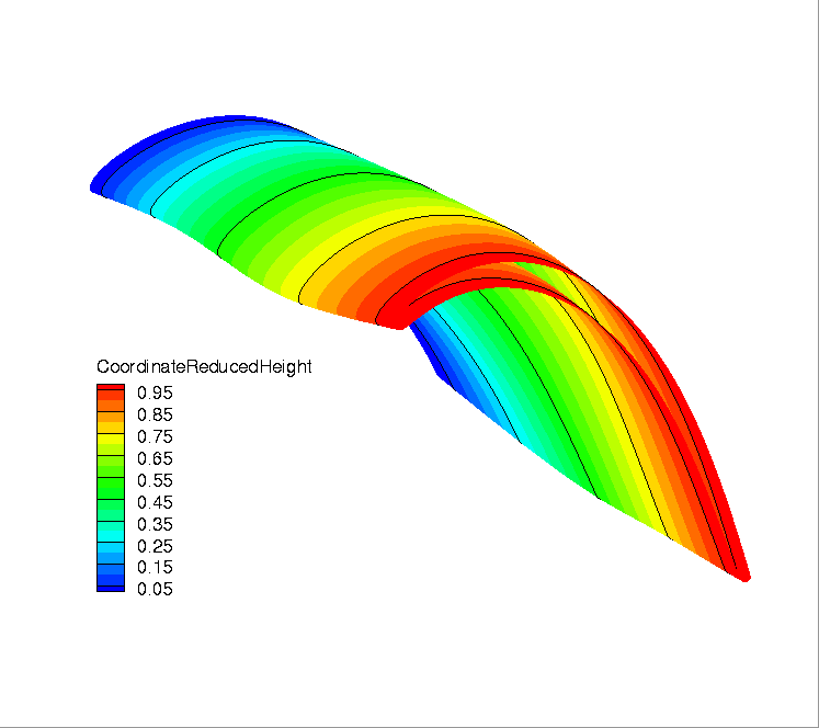
Location of heights on the blade.

for hoH_val in [0.05, 0.25, 0.50, 0.75, 0.95]:
    t = antares.Treatment('isosurface')
    t['base'] = row_1_blade_1
    t['variable'] = 'CoordinateReducedHeight'
    t['value'] = hoH_val
    result = t.execute()

    writer = antares.Writer('hdf_cgns')
    writer['base'] = result
    writer['filename'] = os.path.join('all_iso.cgns')
    writer['append'] = True
    writer['base_name'] = '%s' % hoH_val
    writer['dtype'] = 'float32'
    writer.dump()

‘CoordinateReducedHeight’ corresponds to the h/H variable. Note the option ‘append’ of the writer to concatenate results in a single file.

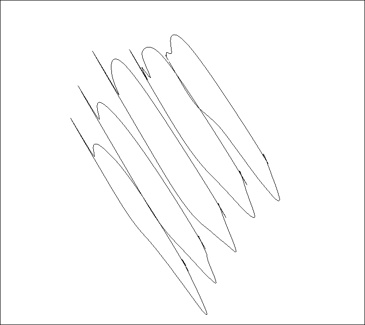
Pressure plots on the five blade profiles.